Python vs. Pine Script Backtesting: Why the Same Trading Strategy Produces Different Results
A Bitcoin study of fill timing, sizing, tick versus basis-point costs and account equity, with measured Python results and an explicit Pine Script comparison protocol.
The same trading signals do not guarantee the same backtest: order timing, quantity, slippage units and open-position accounting can change the result. Our fixed BTC-USDT daily breakout returned +24.46% after modeled costs in 2024–2025, versus +96.28% for a comparable hold account. We quantify four execution conventions in Python, reconcile a losing trade and cross-check every evaluation candle against the exchange API. The Pine implementation discussed here was not run in TradingView; the cross-engine comparison remains unverified.
WHAT THIS STUDY EXPLAINS
- How fixed trading rules connect signals, orders, fills and cash accounting.
- Measured effects of next-open versus same-close fills, signal-time sizing and ticks versus basis points.
- Gross and net results, drawdown, benchmark, all nine development variants and two walk-forward folds.
- How to define a Pine comparison contract and normalize exported records before comparing engines.
The trading rule is only one part of a backtest
Two implementations can agree that Bitcoin broke out and still disagree about how many units were bought, what the fill cost and which profit number to report. A close-time signal is an instruction to create an order. It is not a record that the order filled at that close. TradingView normally processes an ordinary market order on the next available tick, commonly the next bar’s open; settings can change that policy. [1]
We investigate those differences with one fixed daily Bitcoin breakout rule. Four declared execution conventions run against exactly the same candles. All numerical comparisons below were executed in Python. The Pine Script implementation discussed here was not compiled or run in TradingView, and there is no exported Pine ledger in this study. We therefore measure the consequences of specified conventions, rather than claiming a completed cross-platform performance test.
| Python calculation | Quantity and fill policy | Evaluation return |
|---|---|---|
| reference-next-open | 90% of cash including fee, sized at the next open; 5 bp adverse fill | +24.46% |
| signal-qty-bps | Quantity fixed using the signal close; next-open fill with 5 bp adverse adjustment | +24.47% |
| signal-qty-ticks | Same signal-time quantity; next-open fill with five 0.01-USDT ticks | +25.13% |
| same-close | Fill at the completed signal close with 5 bp adverse adjustment; a timing counterfactual | +24.46% |
This extends our worked algorithm-building study. That article established a complete research workflow and discussed Pine sizing and slippage differences. Here those differences become explicit experiments. The final section explains how to compare records from your own Python and TradingView implementations.
Fix the economic question and the accounting before running it
The economic hypothesis is that persistent trends may repay repeated failed breakouts. It does not imply that 55 and 20 are uniquely profitable numbers. We keep those lookbacks from the earlier article so the execution investigation has a stable object. Choosing a new rule because its equity chart looks attractive would answer a different question and add another selection opportunity.
| Item | Recorded convention |
|---|---|
| Market and data | BTC-USDT spot prices, daily UTC bars; 2020-02-20–2025-12-31 input |
| Entry | When flat: completed close strictly above the highest HIGH of the preceding 55 bars, excluding the current bar |
| Exit | When long: completed close strictly below the lowest LOW of the preceding 20 bars, excluding the current bar |
| Orders | Signal after close; fill on the following open; final-bar orders remain unfilled |
| Capital | 10,000 USDT at each period start, flat; 90% cash budget including entry fee, fractional BTC |
| Primary costs | 10 bp commission plus 5 bp adverse price adjustment on each side |
| Other assumptions | No leverage, shorts, funding, cash interest, tax or fixed operating costs; no separate spread charge |
| Final position | Mark at final close; no forced sale and no hypothetical exit-cost reserve |
| Periods | Development 2021–2022; validation 2023; evaluation 2024–2025; earlier data warms indicators |
We recorded the specification, configuration and data amendment before this workflow’s performance calculation. This is an internal research record, not independent preregistration. The same rule and overlapping market history were already studied on this site. The 2024–2025 segment is a chronological evaluation of the frozen implementation, not fresh evidence from previously unknown markets.
The primary acceptance condition is mechanical: fills follow the recorded information timing, cash never borrows and closed plus open profit reconciles to account equity. For economic assessment we report the same-budget hold baseline, drawdown, friction sensitivity and profit concentration. A positive return alone does not pass a deployment decision.
What the new source check establishes
The primary calculation uses 2,142 daily observations from the dataset used in our earlier study: six four-hour candles aggregated into each UTC day, published by humblefool06 on Hugging Face under a CC BY 4.0 declaration. Our research records retain the pinned revision, attribution, transformation note and SHA-256 hashes. The retained series begins on 20 February 2020, after the earlier study excluded an incomplete preceding day. This analysis uses the fixed subset ending 31 December 2025. [3] [9]
We separately retrieved all 731 daily candles for 2024–2025 through Binance’s public market-data API. All 3,655 open, high, low, close and volume comparisons matched exactly. The verification report records request URLs, response hashes and the comparison procedure. The raw API response is not redistributed as the primary dataset. Binance documents UTC as the default candle boundary and identifies klines by opening time. [4]
That is stronger than checking a file hash alone: it tests whether another delivery route reports the same evaluation candles. It remains a same-exchange cross-check, not an independent price audit, and it does not establish that an order could have traded at an OHLC value. Warm-up and development history were not covered by this 731-candle API comparison.
When loading the research data, we checked timestamp continuity, duplicate dates, finite positive prices and OHLC consistency. A reproducible wrong series would still be wrong; the source card and the verification procedure described here expose that residual uncertainty. We do not invent an expert reviewer or a second independent feed to strengthen the presentation.
A completed signal cannot buy the earlier open
The reference loop first executes yesterday’s pending order at today’s open, then values the position at today’s completed close, and only then computes today’s next instruction. The entry and exit channels contain earlier bars only. Including today’s high in an entry channel would make a strict close-above-high breakout impossible on valid OHLC data. For tests of information availability, see our look-ahead-bias investigation.
entry_level = max(b.high for b in bars[i-55:i])
exit_level = min(b.low for b in bars[i-20:i])
# Evaluate only after today's completed close.
if quantity == 0 and bar.close > entry_level:
    pending = ("buy", bar.date)
elif quantity > 0 and bar.close < exit_level:
    pending = ("sell", bar.date)
# Execute pending on the next bar; never at this bar's earlier open.
At the fill, the cash-allocation reference buys q = 0.9 × cash / [fill × (1 + fee)]. A broker or simulator can calculate that quantity when the execution price is known. A Pine order with explicit quantity submitted at the preceding close must use information available then. Our alternative fixes quantity using the signal close and rejects a later unaffordable order instead of inventing cash or resizing it silently.
A synthetic gap makes the difference easy to inspect: with 10,000 USDT, a signal close of 100 and next open of 110, zero costs and a 90% allocation, fill-time sizing buys 81.818182 units and leaves 1,000 cash. Signal-time sizing requests 90 units, spends 9,900 and leaves 100. Both accounts start at 10,000 equity at the fill; their subsequent exposure differs. This arithmetic example is illustrative, separate from the measured Bitcoin history.
Make the Pine contract explicit before comparing its returns
The Pine v6 design considered here uses confirmed daily bars, prior-bar channels, explicit signal-time quantity, percentage commissions and five ticks of native slippage. An independent comparison should use a standard BTCUSDT spot daily chart, the date window in our fixed specification, sufficient warm-up history and the stated settings. There is no TradingView compilation or Strategy Tester validation in this investigation.
Two units are easily confused: five basis points means 0.05% of price, while five ticks of 0.01 USDT means 0.05 USDT. At a hypothetical 100,000-USDT Bitcoin price they imply 50 USDT and 0.05 USDT of adverse adjustment respectively. A tick count is not a percentage. Pine’s built-in slippage accepts ticks, and an explicit entry qty overrides default percentage sizing. [1]
The signal-qty-ticks Python model is a reconciliation target for the stated Pine conventions, not a complete replica of TradingView. Feed revisions, minimum contract increments, quantity rounding, affordability and margin rules can still differ. The reference permits fractional units without exchange lot filters; none of these simulated quantities is a claim of venue-valid live orders.
Keep calc_on_every_tick and calc_on_order_fills at their declared defaults and process_orders_on_close disabled. Changing the calculation or order-processing policy changes the experiment. Pine’s execution model distinguishes historical and realtime updates, so a strategy that appears equivalent on completed candles can behave differently while a candle is still forming. [2]
The reference made money and still failed the return benchmark
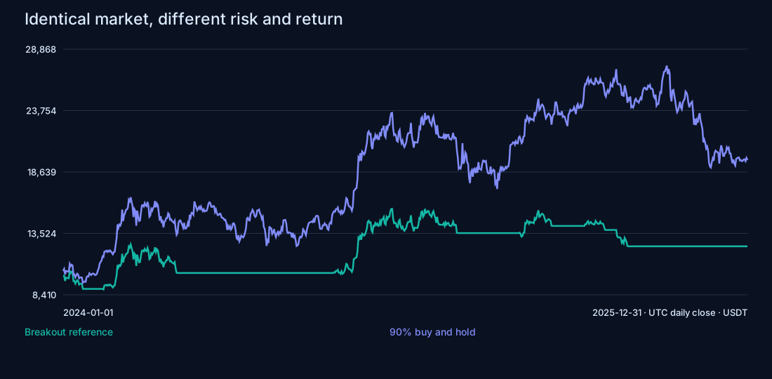
Across the 731 evaluation days from 1 January 2024 through 31 December 2025, the reference turned 10,000 into 12,445.81 USDT: +24.46% after assumed variable costs. The comparable initial-allocation hold account returned +96.28%. These are cumulative returns for the stated interval, not annualized figures.
| Period | Days | Gross strategy | Net strategy | 90% hold | Closed trades |
|---|---|---|---|---|---|
| 2021–2022 development | 730 | +22.64% | +21.32% | -38.60% | 4 |
| 2023 validation | 365 | +17.97% | +16.55% | +139.71% | 4 |
| 2024–2025 evaluation | 731 | +26.50% | +24.46% | +96.28% | 6 |
The strategy’s maximum daily-close drawdown was 20.04%, versus 30.86% for hold. Its mean marked invested exposure was 37.59%, with a position on 300 of 731 closes. Total traded notional divided by initial equity was 12.96 times; this turnover measure counts both buys and sells, not round trips.
Hold carries the initial allocation through the full interval while the breakout strategy moves between cash and Bitcoin. Higher return with higher drawdown is not a complete risk-adjusted ranking. The concrete conclusion is narrower: the breakout account did not beat the specified cumulative-return benchmark. Daily-close drawdown also omits losses that occurred and recovered within a day.
Audit a losing trade from order to cash balance
The first losing closed evaluation trade entered on 2024-01-03, after the signal on 2024-01-02, and exited on 2024-01-23, after 2024-01-22. Its quantity was 0.19993623 BTC. The ledger records the raw reference price separately from the adversely adjusted fill; the table below uses actual simulated fills.
Entry notional was 8,991.01 USDT and entry commission 8.99. Cash fell from 10,000.00 to 1,000.00. At exit the position’s fill-price P&L was -1,083.88; deducting both commissions gives -1,100.78 USDT net. The ending cash was 8,899.22. Tiny apparent differences when adding displayed values come from rounding; the research calculations retain full precision.
| Ledger item | Value |
|---|---|
| Entry fill | 44,969.38 |
| BTC quantity | 0.19993623 |
| Entry fee | 8.99 |
| Cash after entry | 1,000.00 |
| Exit fill | 39,548.24 |
| Exit fee | 7.91 |
| Fill-price P&L before commissions | -1,083.88 |
| Net closed-trade P&L | -1,100.78 |
| Cash after exit | 8,899.22 |
Slippage has already changed the entry and exit fill prices. Deducting the displayed slippage shortfall again from fill-price P&L would charge it twice. “Gross trade P&L” in this ledger means before commissions but after fill-price slippage; the separate gross strategy run removes both fees and slippage. Those labels describe different calculations.
Closed-trade profit and account equity answer different questions
The evaluation ends flat, so its six closed trades explain the entire account profit. The 2023 validation account provides the more revealing example: closed trades lost 669.03 USDT while the remaining 0.25356187 BTC carried 2,323.63 of open marked profit, after deducting its paid entry fee. Total account profit was therefore 1,654.60 USDT, or +16.55%. Ending cash was only 933.10; inventory made up the rest of the 11,654.60 account value.
The reconciliation identity is initial equity + closed net P&L + open marked P&L = cash + marked inventory = ending equity. We check it at full precision for each run. A platform’s closed-trade statistic can disagree with total account return even when both are arithmetically correct. Compare like quantities before treating that disagreement as a bug.
A final-close liquidation would answer another question and incur another sale fee and adverse fill. We retain the open mark and disclose the convention instead of silently switching between realized and unrealized results.
Which execution difference matters on these candles?
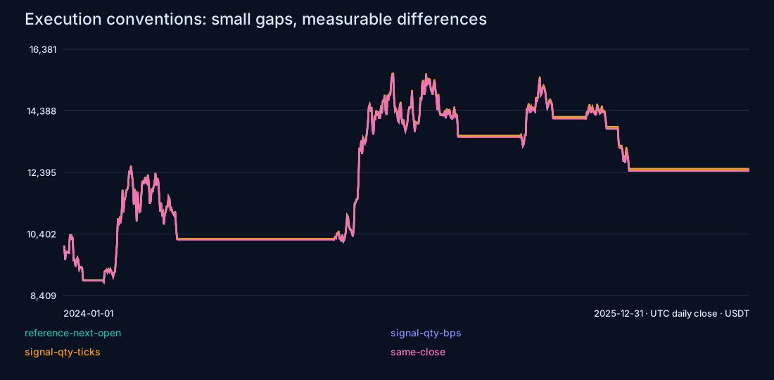
Changing only sizing from fill-time cash allocation to a fixed signal-close quantity moves evaluation return by +0.0099 percentage points. Switching that quantity model from five basis points to five ticks changes return by +0.6651 points, or 66.507521 USDT. Same-close execution changes the reference ending balance by just +0.002848 USDT. These are measured policy effects in Python, not observed TradingView discrepancies.
Bitcoin trades continuously, so adjacent daily closes and opens in this sample can be close together. A small timing effect here does not make same-close fills valid for another market, an illiquid interval or a live implementation with latency. The synthetic gap example shows why the same programming choice can matter much more under other price paths.
When reconciling implementations, compare their fill records before comparing equity curves. Find the first differing quantity or price, then follow its cash effect forward. Differences compound: later allocations depend on earlier cash. Similar final returns do not prove matching trade mechanics.
Test costs and dependence on exceptional trades
The reference paid 129.58 USDT in commissions across 12 fills. The cost table keeps commission at 10 bp per side and varies the adverse price adjustment. Zero adverse adjustment here is not a zero-cost account; the gross strategy row in the earlier table is the separate no-fee, no-slippage calculation. The assumptions combine spread and execution shortfall into one adverse adjustment, rather than estimating a historical bid/ask spread. For broader fee categories, see our trading-cost analysis.
| Commission per side | Adverse adjustment per side | Net return | Max daily-close drawdown |
|---|---|---|---|
| 10 bp | 0 bp | +25.13% | 19.79% |
| 10 bp | 5 bp | +24.46% | 20.04% |
| 10 bp | 10 bp | +23.79% | 20.30% |
| 10 bp | 20 bp | +22.45% | 20.80% |
Average closed-trade net P&L was 407.63 USDT. The average winner was 1,748.18 and average loser -932.91; closed-trade profit factor was 1.87, with 50.00% winning trades. Dollar averages depend on the evolving account size. They are descriptive summaries of this ledger, not stable forecasts of the next trade.
The three largest closed trades contributed 5,244.53 USDT. Subtracting those contributions from total account P&L leaves -2,798.72. That arithmetic stresses concentration; it is not a rerun in which the trades were skipped and later position sizes recomputed. Annual returns also show the path: 2024 +38.44%; 2025 -10.10%. Calendar returns come from the continuous evaluation account, rather than fresh annual accounts.
Keep the rejected variants where readers can see them
We declared nine combinations: entry lookbacks 35, 55 and 80, each with exit lookbacks 10, 20 and 30. The table reports every development result after costs. We keep 55/20 regardless of its ranking, so the comparison does not quietly become a search for the most flattering execution headline.
| Entry lookback | Exit 10 | Exit 20 | Exit 30 |
|---|---|---|---|
| 35 | +4.00% | +10.03% | -9.22% |
| 55 | +14.61% | +21.32% | +17.48% |
| 80 | +9.12% | +15.55% | +11.89% |
Eight of nine cells are positive, but returns range from −9.22% to +21.32%; the 35/30 combination loses and exit settings change the result substantially. The retained 55/20 rule also happens to rank first. Its selection record precedes this run, but the earlier article already familiarized us with the rule: this coincidence is not independent confirmation. Shared market history makes these correlated results, and neither a split nor a grid erases prior knowledge. Bailey and coauthors analyze how backtest selection can overfit; our grid is not their formal probability-of-backtest-overfitting estimator. [5]
The two walk-forward folds test a documented selection procedure using only earlier data: choose the best of those nine by training return, then evaluate the next year. They use 2022 and 2023 as test folds and never select using 2024–2025. These folds are diagnostic extensions, not additional untouched evidence for the final account.
A selection procedure must survive its next period
Each fold restarts with 10,000 USDT, uses earlier bars for indicator warm-up and applies the selected parameters without further modification. A favorable training rank gives a candidate permission to be tested; it does not supply the test result.
| Training period | Next test year | Selected entry/exit | Test net return |
|---|---|---|---|
| 2021-01-01–2021-12-31 | 2022 | 35/20 | -30.54% |
| 2021-01-01–2022-12-31 | 2023 | 55/20 | +16.55% |
We retain both the selected parameters and the subsequent return. If a later period loses, that failure remains in the report. We do not add new filters, retune the primary rule or keep opening the final period until the article obtains a winning result.
Monte Carlo paths change the ordering, not the amount of evidence
We resample the reference account’s 731 observed daily net equity returns in circular contiguous 20-day blocks, wrapping at the end of the series. Each simulated path contains the same number of days and starts with the same capital. The fixed seed is 6142026; 5,000 paths make the calculation reproducible. Blocks preserve some local serial dependence, unlike shuffling individual days. The block length is an explicit modeling choice, not an estimated optimum. [6]
The simulated median cumulative return was +20.98%, with 5th and 95th percentiles -38.34% and +166.29%. Median maximum drawdown was 30.22%; the 95th percentile was 50.12%. The fraction of losing simulated paths was 32.28%. These are conditional path summaries, not a calibrated probability of future loss or a confidence interval for alpha.
Resampling account returns does not generate new candles, rerun the breakout decisions, model new liquidity conditions or restore missing crises. We do not bootstrap benchmark-relative performance here. More simulated paths reduce Monte Carlo noise around this chosen procedure; they leave the underlying historical evidence at the same 731 days and the same trade sequence.
Give the assistant a testable task at each stage
ChatGPT and Claude can help articulate a rule, explain an accounting discrepancy and challenge a report. Codex and Claude Code can inspect a repository, edit its files and run development commands. Those documented capabilities support the workflow; they do not demonstrate a profitable trading algorithm. This investigation used Codex for repository development and Python for calculations. We did not run a controlled ChatGPT-versus-Claude experiment or use either assistant to forecast the trading signals. [7] [8]
First settle the information boundary. An assistant should expose unresolved details before it implements them: strict or inclusive comparison, earlier-bar windows, order timing, cash budget, rounding and final inventory. The first prompt is a reusable brief, not a claim that we recorded a model-comparison experiment.
Turn this trading idea into an executable specification before coding. State the economic hypothesis; entry and exit; which bars each input uses; signal availability; order and fill timing; quantity and cash constraints; costs; timezone; end valuation; chronological periods; benchmark; and decision criteria. List unresolved choices. Do not select rules because they improve historical results.Then constrain implementation. Ask for a state machine and fixtures, with no strategy optimization hidden inside a request to fix a bug. A useful future-data test changes prices after date t and checks that no earlier decision or fill changes. A useful accounting test reconciles cash, inventory and fees even when the final trade remains open.
Implement the attached frozen specification exactly. Separate signals, order creation, fills, cash accounting and reporting. Do not add filters or optimize parameters. Use synthetic fixtures for current-bar exclusion, next-open timing, fee-inclusive sizing, unaffordable orders and an open final position. Show the mapping from each rule to code and test.For debugging, compare rows from the first divergence. For reporting, require file-derived figures and explicit status labels for unexecuted components. Market data supplies observations, executable code performs the calculation, and the researcher decides which assumptions and comparisons deserve confidence.
Compare these two normalized ledgers in timestamp order. Find the earliest difference in input bar, signal, requested quantity, fill price, commission, position or equity. Explain it using the recorded settings and row values. Reconcile initial equity plus closed and open P&L to ending equity. Do not retune the strategy or infer a bug from final return alone.Generate the report only from the supplied configuration, data manifest and executed result files. Include all tested variants, period boundaries, gross and net returns, benchmark, drawdown, exposure, turnover, trade concentration and open-position accounting. Link every table to its source file. Mark unexecuted code and unavailable checks explicitly. Preserve unfavorable results; do not invent a review or model comparison.How to check your actual TradingView run
To compare your own Pine and Python implementations, use a standard daily chart for the same symbol and period, then retain the Pine source, settings, chart feed and exported trades. Start with the zero-cost case when isolating signals, then add commissions and the same tick-based slippage to both engines. Compare signal dates and trades before comparing account returns. Differences in lot increments or feed history should be documented as mismatches rather than rounded away.
Normalize both sets of fill records to a shared schema: timestamp, side, requested quantity, reference price, fill price, commission, resulting position, cash and equity. Map each export field explicitly, including its timezone, units and rounding. Compare against the signal-quantity, tick-cost Python convention described here. This is a diagnostic protocol, not a claim that every localized Strategy Tester export has the same format. Without an exported Pine run, the cross-engine result remains unverified.
This sequence also explains why a profitable backtest can lose live: the live system may receive different candles, create a later order, fill fewer units or pay a different spread. Once those records agree, a remaining performance failure becomes a question about the strategy and market, rather than an excuse to keep changing execution assumptions.
Before trusting matching backtest returns
- Match the instrument, feed, UTC candle boundaries, date window and indicator warm-up.
- Record the exact order timing, quantity formula, tick size, commission and affordability policy.
- Compare the first divergent fill before comparing the final balance.
- Reconcile closed profit, open inventory, fees, cash and marked equity.
- Keep every declared variant and distinguish reused history from new prospective evidence.
- Freeze the next forward test; retain signals, submitted orders and confirmed fills.
Practical questions
Why do Python and Pine Script backtests differ?
The programming language is rarely a sufficient explanation. Data, signal availability, order timing, sizing, costs and account definitions determine the result. This investigation changes those conventions explicitly in Python and describes a Pine comparison protocol for separately exported records.
Can ChatGPT or Claude build a profitable trading bot?
They can help build and inspect the code. Our reference produced +24.46% after assumed variable costs in the stated historical period, but that does not show either assistant added an investment edge. No comparative AI investment experiment or live profitability test was conducted.
How do I know whether a strategy has an edge?
First establish that the code implements its intended information and accounting rules. Then evaluate its frozen selection procedure against a suitable benchmark, realistic costs and later observations. Profit concentration, prior research choices and changes in execution all affect the interpretation; one positive backtest cannot settle them.
How do I avoid overfitting trading strategies?
Document every attempt, limit discretionary variations, separate chronological selection and evaluation, and preserve losing variants. The nine-cell grid and two walk-forward folds here expose sensitivity; they do not certify that the surviving rule is robust or erase knowledge from the earlier study.
Does Monte Carlo simulation prove a trading advantage?
No. This block bootstrap rearranges observed daily net account returns under a declared dependence assumption. Its paths help inspect conditional drawdown and return sensitivity. They do not create new historical data, generate new market regimes or establish predictive value.
Is the Pine Script strategy validated against Python?
No. The Python calculations and tests were executed. The Pine companion was not compiled or run in TradingView; it uses signal-time quantity and fixed-tick slippage. Its actual exported fills still need comparison with the stated Python target.
Sources and methodology
Tables and charts are our executed calculations from the attributed input, not findings reported by the sources below. Our research process recorded the protocol, pre-calculation amendments, source hashes, API cross-checks, tests and signal-to-equity accounting. The article presents the assumptions and measured results needed to assess the argument. External documentation supports platform behavior and methods; it does not endorse the strategy. No independent expert review is claimed.
- TradingView: Pine Script strategies and broker emulator
- TradingView: Pine Script execution model
- humblefool06: BTC-USDT four-hour dataset and source card
- Binance: public spot kline market-data documentation
- Bailey et al.: The Probability of Backtest Overfitting
- Politis and White: Automatic Block-Length Selection for the Dependent Bootstrap
- OpenAI: code generation and Codex
- Anthropic: Claude Code overview
- Creative Commons: Attribution 4.0 terms
Retrospective educational research using modeled variable costs. Taxes and fixed operating costs are excluded. No live execution, TradingView performance run or comparative AI investment experiment was conducted.