How to Build a Trading Algorithm with ChatGPT or Claude—and Test Whether It’s Profitable and Avoid Overfitting
A reproducible Python and Pine Script trading project: exact rules, actual backtest results, costs, walk-forward tests and Monte Carlo analysis to examine overfitting.
Yes, ChatGPT or Claude can help you build a trading algorithm, and the resulting strategy can make money. In our worked Python study, a fixed Bitcoin breakout rule returned 11.55% after modeled trading costs from 1 January 2024 through 31 July 2026. It also suffered a 29.72% daily-close drawdown and earned less than a comparable initial-allocation buy-and-hold baseline. Those are actual retrospective calculations, not a forecast or evidence that an AI provider has a trading edge. This article explains the rules, calculations, trade accounting and tests used to examine that distinction.
WHAT YOU WILL LEAVE WITH
- A fully specified 55-day breakout / 20-day exit strategy, its Python accounting model and an explanation of the Pine Script differences.
- Actual results, including losing trades, commissions, an open-position accounting example and a buy-and-hold comparison.
- All nine development variants, four walk-forward folds and 15,000 conditional bootstrap paths—not a handpicked equity curve.
- Reusable prompts for ChatGPT, Claude, Codex and Claude Code, with concrete acceptance conditions for their work.
- A clear answer to what this study establishes, what it leaves unresolved and what a prospective test should record.
A complete trading research project, with an answer you can inspect
“Build me a profitable trading bot” combines three jobs: inventing a rule, implementing it and establishing whether it deserves capital. An assistant can produce persuasive code while leaving the first and third jobs unresolved. We separate them here by fixing a simple strategy, executing a documented historical study and publishing the records behind the result.
The project is a daily, long-only Bitcoin breakout system. Its economic hypothesis is modest: sustained trends may occasionally repay the cost of repeated failed breakouts. The uncomfortable part is integral to the idea. A trend follower can lose on most trades and depend on a few large winners. We therefore examine the distribution of trade P&L as well as the account’s final balance.
The investigation separates the strategy rules, market observations, simulated fills and account results. We retain the source attribution, daily input, 15 executable tests and complete experiment records. The sections below explain the calculations and show the consequential trade and accounting examples.
This is an AI-assisted engineering study, not an experiment in asking a chatbot which asset will rise. The code was developed in Codex. We did not run the same task through ChatGPT and Claude, measure their investment performance or use a language model to choose trades at runtime. Once written, the algorithm follows deterministic rules.
For a focused reconciliation exercise, continue with Python vs. Pine Script backtesting: why results differ.
Start with a specification that leaves no profitable ambiguity
A strategy description should settle the details that can change the trade list. “Buy the 55-day high” is insufficient: does a wick count, does the current bar belong in the channel, and can a completed daily candle somehow be bought at its earlier opening price? Our rule requires a completed close above earlier highs, then waits for the following open.
The specification and evaluation procedure were written before this workflow calculated performance. Two data amendments came first: a source replacement and a response to a missing four-hour observation. Both are preserved in the research records. We did not change the trading rule to improve its result. This record is an internal sequence of research decisions, not an independently timestamped preregistration or a prospective experiment.
| Component | Exact rule |
|---|---|
| Instrument and clock | BTC-USDT; six four-hour observations aggregated into each UTC daily OHLC bar. |
| Entry | When flat, completed close > highest HIGH of the preceding 55 daily bars; exclude the current bar. |
| Exit | When long, completed close < lowest LOW of the preceding 20 daily bars; exclude the current bar. |
| Fill timing | Signal at close; buy or sell at the next daily raw open, adversely adjusted for slippage. |
| Position | One long position, fractional BTC, no leverage or short selling; exit the entire position. |
| Entry budget | 90% of available cash including entry commission; quantity = 0.9 × cash / [fill price × (1 + commission rate)]. |
| Primary costs | 10 basis points commission plus 5 basis points adverse slippage EACH SIDE; assumed, not current venue quotes. |
| Account boundary | Start each reported period flat with 10,000 USDT; earlier bars warm indicators only. |
| End valuation | Mark at the final daily close; no forced liquidation and no hypothetical exit-cost reserve. |
| Excluded costs | Taxes, fixed subscriptions, data and hosting; no cash interest, funding or borrow charges. |
The assumed execution boundary is idealized. The completed daily close and the next daily open are adjacent in a continuous crypto market; an actual implementation takes time to receive data, calculate and submit an order. Five basis points of slippage is an assumption, not evidence that this latency and order size can be executed at that price.
The data inspection changed the study before the backtest began
The input is a third-party BTC-USDT archive published by humblefool06 on Hugging Face under a CC BY 4.0 declaration. We pinned revision 9f491eb5340dd6a24f27fde24edf098e1e785443, retained the publisher’s dataset card and recorded SHA256 hashes. TensorParadigm aggregated the four-hour candles to UTC daily bars. We recorded this attribution and transformation in the research records. [1] [9]
Coverage checks found that 19 February 2020 lacked its 12:00 UTC component. We excluded that day and all earlier history rather than invent a price. The normalized input consequently starts on 20 February 2020; development starts on 1 May, after 71 complete warm-up bars. All 2,354 retained daily observations contain exactly six components. Timestamp ordering, duplicates, finite values and OHLC consistency were checked before performance.
A hash identifies the bytes used; it does not establish that the publisher’s prices are correct. We have not independently reconciled this third-party archive to exchange records. A stronger investment study would repeat the analysis on an independently obtained feed and investigate discrepancies. Reproducibility and source accuracy are related but different requirements.
| Segment | Dates | How it is used |
|---|---|---|
| Development | 1 May 2020–31 December 2022; 975 days | Report the fixed rule and all nine prespecified parameter variants. |
| Validation | 1 January–31 December 2023; 365 days | Report the unchanged 55/20 rule; do not use it to revise the primary parameters. |
| Reserved historical evaluation | 1 January 2024–31 July 2026; 943 days | Main fixed-rule result and bootstrap input. |
| Secondary walk-forward | 2023, 2024, 2025 and January–July 2026 | Select with earlier data, then evaluate the next fold; overlaps the segments above. |
We reserve “reserved historical evaluation” for the fixed rule’s last segment. It is historical data from a market whose broad history is already known. Moreover, the secondary walk-forward exercise later reuses overlapping dates. There is no globally untouched final sample across every analysis in this article. Calling it an independent live test would overstate the design.
Ask the assistant to remove ambiguity before writing the trading bot
ChatGPT and Claude can help translate a research brief into code, explain a ledger and propose tests. Codex and Claude Code can work within a codebase, edit files and run commands. Their documented engineering capabilities justify trying them on this workflow; they do not establish which product writes the most profitable strategy. [3] [4]
Give the assistant the fixed specification and require it to name unresolved choices before implementation. In this study, the important choices include strict versus inclusive breakouts, prior-bar windows, next-open execution, the fee-inclusive cash budget and treatment of an open final position. A confident answer that silently invents any of these is a defective implementation.
Implement the attached fixed strategy specification. First identify any ambiguity that could change signals, fills, sizing or reported P&L. Do not add filters or optimize parameters. State when each input becomes available. Separate signal logic, execution, accounting and reporting. Before running historical performance, create synthetic tests for timing and cash reconciliation. Return the complete code, assumptions and an experiment log.The prompt below is a reusable research brief, not a transcript of a controlled model comparison. Keep an experiment log containing the model/version, supplied files, accepted changes and every subsequent strategy variation. Otherwise “one idea” can quietly become dozens of unrecorded opportunities to discover a flattering backtest.
Build the Python backtest around the order of events
The engine’s daily loop has a deliberate order: execute yesterday’s pending order at today’s open, mark the account at today’s close, then calculate today’s decision. This prevents a daily close from being used to obtain a fill earlier in the same candle. Both channels exclude the decision bar. These abbreviated excerpts show the two calculations most likely to be implemented incorrectly.
# Called at the completed close, after any pending open fill.
entry_level = max(b.high for b in bars[index-entry_lookback:index])
exit_level = min(b.low for b in bars[index-exit_lookback:index])

if not quantity and bar.close > entry_level:
    pending = {"side": "BUY", "signal_date": bar.date}
elif quantity and bar.close < exit_level:
    pending = {"side": "SELL", "signal_date": bar.date}
# Execute pending only on the NEXT loop iteration, at that bar's open.
Entry sizing includes the commission inside the 90% budget. With commission c and adverse buy fill P, quantity is 0.9 × cash / [P × (1 + c)]. Deducting a fee after buying 90% of cash would spend more than the specified budget. Slippage is already reflected in P; subtracting its estimated cash value again would charge it twice.
commission = commission_bps / 10000
slippage = slippage_bps / 10000
fill_price = bar.open * (1 + slippage)  # adverse BUY fill
qty = allocation * cash / (fill_price * (1 + commission))
notional = qty * fill_price
fee = notional * commission
cash -= notional + fee
We ran 15 synthetic tests. They cover future-data perturbation, current-bar exclusion, strict breakouts, next-open fills, adverse slippage, fee-inclusive sizing, closed P&L, open equity, the same-budget baseline, final unfilled signals, warm-up isolation, invalid data and bootstrap arithmetic. These tests establish particular timing and accounting properties. They do not establish a market edge.
One useful invariant is more revealing than an attractive chart: changing prices after date t must not change a decision or fill before t. Another is exact reconciliation, within floating-point tolerance: initial equity + closed-trade net P&L + marked open-position P&L = ending equity. The runner checks this identity for every account it simulates.
A Pine Script implementation, with disclosed differences
We also wrote a Pine Script implementation of the same prior-channel entry and exit idea on a standard daily chart. It uses confirmed bars and schedules ordinary orders for the next bar. TradingView’s strategy broker emulator and its settings determine simulated fills; chart data and intrabar assumptions can matter. [2]
We did not compile this companion in TradingView or obtain a Strategy Tester result. Every performance number in this article comes from the Python engine. The Pine source has been reviewed as code, which is a narrower check than running it.
There are two intentional non-parities. Pine’s slippage setting uses a fixed number of ticks, whereas Python uses five basis points proportional to price; our Pine version uses zero ticks and therefore does not reproduce the primary cost model. Pine’s native 90%-of-equity sizing also differs from our entry-fee-inclusive 90%-of-cash budget. These differences prevent a claim of equivalent account returns.
For a proper cross-engine comparison, first align the feed, UTC boundaries, warm-up history, date window, quantity convention and fees. Compare the signal dates and fill ledger before comparing returns. If the trades differ, a similar final balance is an accidental agreement rather than validation.
The actual result: profitable in the sample, below the hold baseline
The fixed algorithm turned 10,000 USDT into 11,154.96 USDT in the 943-day reserved period. Its 11.55% return is cumulative for that interval, not annualized. Maximum drawdown measured at daily close was 29.72%. It closed eight trades, won three and finished flat. The positive net result therefore does not depend on an unrealized final position in this particular segment.
The baseline invested 90% of its initial cash, including entry commission, at the first period open and held. It returned 43.66% with a 51.05% daily-close drawdown. It did not rebalance continuously to 90%. The strategy had a mean daily invested exposure of 33.62%; the baseline remained invested and its allocation drifted. Lower drawdown alongside lower return is a tradeoff, not evidence of alpha or a risk-matched comparison.
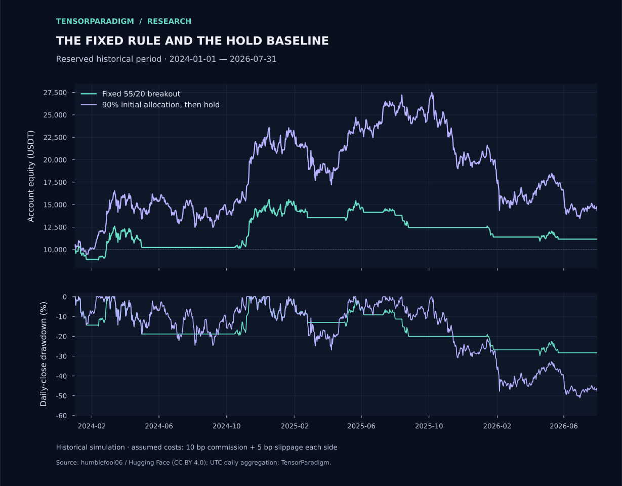
Each column below is a separate account starting flat. Do not compound the three returns into a continuous track record: the resets and end positions differ. The lengths also differ, so the percentages cannot be compared as annual rates.
| Metric | Development: May 2020–2022 | Validation: 2023 | Reserved: Jan 2024–Jul 2026 |
|---|---|---|---|
| Net account return | +170.39% | +16.55% | +11.55% |
| Ending equity, USDT | 27,039.04 | 11,654.60 | 11,154.96 |
| Daily-close maximum drawdown | 41.48% | 24.27% | 29.72% |
| Closed trades / open at end | 5 / 0 | 4 / 1 | 8 / 0 |
| Closed-trade win rate | 60.00% | 25.00% | 37.50% |
| Closed-trade net profit factor | 4.05 | 0.66 | 1.28 |
| Mean daily invested exposure | 41.68% | 57.59% | 33.62% |
| 90%-initial-allocation hold return | +82.46% | +139.71% | +43.66% |
| Hold daily-close maximum drawdown | 75.56% | 18.90% | 51.05% |
The 2023 result demonstrates why trade summaries can mislead. Its four closed trades lost 669.03 USDT, yet its account gained 1,654.60 USDT because an open position had 2,323.63 USDT of marked P&L net of entry cost. We reserve no hypothetical exit fee. A closed-trade profit factor of 0.66 and a positive total account return can both be correct.
Audit one losing trade before trusting the winning account
The first reserved-period entry signal occurred on 2 January 2024. The strategy bought at the 3 January raw open of 44,946.91 USDT, adjusted upward by five basis points to 44,969.383455. With a 9,000 USDT total entry budget, it acquired approximately 0.19993623 BTC. Entry notional was 8,991.008991 USDT and commission was 8.991009 USDT.
An exit signal on 22 January led to a 23 January fill. The raw open of 39,568.02 became 39,548.23599 after adverse sell slippage. Sale notional was 7,907.125205 USDT; after 7.907125 USDT commission, proceeds were 7,899.218080 USDT. Subtract the original 9,000 USDT entry cash cost: net loss 1,100.781920 USDT. Together with the untouched 1,000 USDT cash, the flat account then held 8,899.218080 USDT.
| Record | Value |
|---|---|
| Entry signal → fill | 2 January → 3 January 2024 |
| Entry fill / BTC quantity | 44,969.383455 / 0.19993623 |
| Entry notional + commission | 8,991.008991 + 8.991009 = 9,000.000000 USDT |
| Exit signal → fill | 22 January → 23 January 2024 |
| Exit notional − commission | 7,907.125205 − 7.907125 = 7,899.218080 USDT |
| Net trade P&L | 7,899.218080 − 9,000.000000 = −1,100.781920 USDT |
This ledger is a better implementation check than a rounded percentage. It exposes signal timing, adverse prices, fee bases and the difference between a trade return on committed cash (−12.23%) and the account change (−11.01%). If an assistant cannot reconcile these amounts, further optimization only elaborates an unreliable calculation.
Costs matter, but the concentration of profit matters more here
In the reserved primary run, actual modeled commissions totaled 171.19 USDT. The quantity-weighted adverse price difference from raw opens was 85.59 USDT. The latter is an execution-reference diagnostic: the adverse fills already incorporate it. Summed buy and sell notionals were 17.12 times initial capital, showing why a small per-side cost can accumulate.
We reran the same rules at three assumed cost settings. The zero-cost run earned 13.99%, the primary run 11.55% and the higher-cost run 9.16%. These are separate simulations. Costs alter the quantity bought and the cash available for later reinvestment, so the difference between their final balances is not simply the primary run’s summed commission and slippage.
| Commission / adverse slippage | Net return | Daily-close maximum drawdown |
|---|---|---|
| 0 / 0 basis points | +13.99% | 28.77% |
| 10 / 5 basis points: primary | +11.55% | 29.72% |
| 20 / 10 basis points | +9.16% | 30.66% |
The three winning closed trades earned 5,244.53 USDT; the other five lost 4,089.57 USDT. Net profit was 1,154.96 USDT. That dependence on a few winners may be consistent with trend following, but eight trades provide little evidence about how reliably those winners will recur. Subtracting the best three P&Ls is a concentration diagnostic, not a valid counterfactual account that could have skipped those trades without changing later sizing.
Fixed costs are outside these returns. For a real account, subtract the data, software, model usage and hosting costs actually attributable to the process, then consider taxes under the relevant rules. A deterministic daily rule does not need an LLM API call for every candle. Avoid adding recurring expense to a calculation that ordinary code can perform.
Avoid overfitting by accounting for the search, not admiring the winner
Overfitting often begins before a formal optimizer runs. Try another asset, change the start date, add a filter, inspect the result and keep the attractive version: each choice increases the effective search. A conventional holdout can become development data after repeated inspection. Research on backtest overfitting addresses this selection problem; it does not give a blanket certificate to any workflow that uses a train/test split. [5]
We fixed nine development configurations: entry windows 40, 55 and 70 days, crossed with exit windows 10, 20 and 30 days. The table shows every net return. The primary 55/20 rule remains the primary rule regardless of the ranking. Several configurations generate identical trades, so nine rows are not nine independent confirmations.
| Entry window | Exit 10 days | Exit 20 days | Exit 30 days |
|---|---|---|---|
| 40 days | +140.64% | +164.32% | +123.77% |
| 55 days | +146.06% | +170.39%: fixed primary | +161.82% |
| 70 days | +146.06% | +170.39% | +161.82% |
All nine were profitable in this development interval. That is useful context about this small neighborhood, but it does not establish an optimum or robustness across assets and regimes. The primary’s five closed development trades are a particularly thin basis for a parameter claim. We have not estimated a formal probability of backtest overfitting or a selection-adjusted significance level.
For your own project, preserve the trials that failed to reach the final table. If you inspect the later sample and then change the rule, label the revised strategy honestly: it has used that sample. A new filename does not restore the information barrier.
Review this strategy specification, experiment log and code for look-ahead, repeated test-set use and unrecorded selection. Trace input availability and fill timing. Construct a minimal failing fixture for each suspected implementation bug. Separate bugs from modeling assumptions and investment hypotheses. Do not change parameters to improve performance. Identify which conclusions are unsupported by the sample.Walk-forward testing evaluates a selection procedure—and can still lose
A secondary experiment asks a different question: what if a researcher selected one of the nine variants from past data each year? For each fold, training begins on 1 May 2020 and ends on the preceding 31 December. Select the highest net-return variant, breaking ties by smaller drawdown and then entry/exit lookback order. Evaluate it in the following year without retuning inside that fold. Chronological splitting preserves the direction of information flow. [6]
| Test fold | Training ends | Selected entry / exit | Test net return | Test max DD | Hold return |
|---|---|---|---|---|---|
| 2023 | 31 December 2022 | 55 / 20 | +16.55% | 24.27% | +139.71% |
| 2024 | 31 December 2023 | 55 / 30 | +38.44% | 19.37% | +108.88% |
| 2025 | 31 December 2024 | 55 / 10 | −4.02% | 15.82% | −5.83% |
| January–July 2026 | 31 December 2025 | 55 / 30 | −14.24% | 15.35% | −25.52% |
The selected algorithm lost 4.02% in 2025 and 14.24% in January–July 2026. A selection procedure can be correctly ordered in time and still disappoint. Optimizing past return does not supply evidence that the selected setting will dominate the next market.
Each fold starts flat with 10,000 USDT. These are independently reset test accounts, not one account continuously carrying positions and wealth between years. The 2026 fold is partial. Do not multiply their returns into a live-equivalent track record.
The 2024–2026 test dates overlap the primary reserved historical segment, and later training windows include earlier test years. This is an explicitly secondary diagnostic, not another untouched holdout or an independent replication of the headline result.
Monte Carlo analysis: describe the uncertainty you actually simulated
We use a circular fixed-length block bootstrap, a resampling method for dependent observations. The input is the fixed primary run’s 943 daily net portfolio returns, including cash days and costs. For each block length of 1, 10 and 30 days, we generate 5,000 paths of the same 943-day horizon using seed 20261018. Blocks can wrap from the sample’s end to its start; the last block is truncated to the required length. [7]
Each simulated path compounds the sampled returns and calculates its own drawdown. This does not simulate fresh BTC prices, rerun the breakout signals or recompute trade costs under a new sequence. It rearranges already-observed portfolio returns. A one-day block discards serial ordering; longer blocks preserve local stretches but not the entire historical regime. None adds a crisis absent from the input.
The simulated terminal-loss fractions range from 39.68% to 42.66%. These are conditional outputs of this resampling experiment, not estimated probabilities that the strategy will lose money over the next 943 days. The sensitivity to block length is itself worth retaining rather than selecting the most reassuring column.
| Block length | Terminal return P05 / median / P95 | Max DD median / P95 | Loss fraction | DD ≥20% fraction |
|---|---|---|---|---|
| 1 day | −44.45% / +11.82% / +126.07% | 34.20% / 56.59% | 39.72% | 94.12% |
| 10 days | −41.73% / +10.97% / +124.93% | 32.65% / 53.35% | 39.68% | 93.20% |
| 30 days | −46.51% / +8.87% / +151.72% | 34.38% / 56.34% | 42.66% | 94.60% |
At 5,000 paths, the Monte Carlo standard error for the loss fraction is about 0.69–0.70 percentage points, calculated as √[p(1−p)/5,000]. This measures finite simulation noise. It omits uncertainty about the data source, the trading rule, future regimes and whether the resampling assumptions are appropriate. Running a million paths would shrink simulation noise without providing more market history. Reporting Monte Carlo error separately from the uncertainty being studied is standard simulation practice. [8]
Audit the result, then ask a better next question
The Python implementation uses the standard library to calculate from normalized daily observations. The research records retain period reports, all nine development variants, the secondary walk-forward results and the bootstrap summaries. Source revisions and hashes identify the observations used in those calculations.
A useful audit starts with the reserved-period ending equity of 11,154.96 USDT and the first losing trade described above. Reconcile each signal, fill, commission and cash change before interpreting the final return. Our calculations retain full precision; rounded article tables are presentation, not replacement input for subsequent calculations.
Then decide what evidence your question requires. To investigate feed accuracy, obtain an independent dataset. To investigate execution, record decision time, submission time, acknowledgment, fill price and quantity under realistic order constraints. To investigate a revised parameter-selection process, write the selection rule before evaluating another chronological period. These are distinct experiments and should remain distinct in the log.
Compare the timestamped strategy signals, submitted orders, confirmed fills and reconciled positions in these files. Identify the earliest divergence. Classify it as data, timing, sizing, execution or accounting, and support each finding with record IDs. Do not retune the strategy. Return a reconciliation table and the smallest reproducible example of any bug.If your goal is a trading journal or setup scanner, the same discipline applies. Store the rule version and the timestamped setup before the outcome; retain skipped and rejected signals as well as trades. Ask an assistant to reconcile that diary to the execution ledger and explain discrepancies. A post-trade story is less useful than a recorded decision whose later outcome can be measured.
Use only the setup definitions and information recorded before each decision. Include taken, skipped and rejected signals. Reconcile actual trades to the order ledger. Report adherence, recurring execution errors and outcomes by prespecified setup category. Separate descriptive patterns from evidence sufficient to change a rule. Flag missing records and small samples.Would we call this a profitable trading algorithm?
In the narrow historical accounting sense, yes: the primary reserved-period account earned 1,154.96 USDT after its assumed commissions and slippage. In the stronger investment sense—an algorithm with a demonstrated, repeatable advantage worth deploying—the evidence is insufficient. Eight closed trades on one third-party crypto archive do not establish that claim.
The decision also depends on the mandate. A reader seeking more cumulative return than the hold baseline did not get it in the headline period. A reader unable to tolerate a roughly 30% daily-close drawdown would reject that observed path. Those are evaluations against possible investor requirements, not acceptance thresholds we secretly specified before seeing results.
A useful next step is a frozen prospective paper test, with a start date recorded before signals arrive and a plan for reconciling every decision to the executable market. Record all proposed revisions without silently replacing the tested version. Paper execution still needs realistic assumptions; small live execution, if later chosen, answers additional questions about actual fills and operations.
The practical value of ChatGPT, Claude, Codex or Claude Code is that an individual can build and inspect this research machinery more quickly. The machinery can deliver an unwelcome answer. In this project it produced a profitable historical account, substantial drawdowns, return below the hold baseline and a small number of consequential trades. Publishing those facts is more useful than asking an assistant for a more persuasive description of the strategy.
Before calling your trading algorithm profitable
- Write entry, exit, timing and sizing rules so two independent programmers would produce the same trades.
- Keep source provenance, an immutable data snapshot or hash, and a record of missing observations.
- Prove that changing future data cannot alter earlier decisions.
- Reconcile initial equity plus closed and open P&L to ending equity.
- Include adverse execution assumptions, commissions and the operating costs relevant to your account.
- Show an appropriate baseline and explain differences in exposure and risk.
- Retain every tested configuration, including failed and abandoned attempts.
- Separate parameter selection from later evaluation, and disclose reused test periods.
- Treat simulated loss frequencies as conditional on their model and historical input.
- Freeze the next version before a forward test; reconcile recorded signals with actual or paper fills.
Questions readers actually need answered
Can ChatGPT or Claude code a profitable trading algorithm?
They can help implement, test and debug one. Our fixed algorithm made 11.55% after assumed variable trading costs in the reserved historical period, but underperformed the hold baseline and had a 29.72% drawdown. That supports a narrow statement about this backtest. It does not show that either assistant can reliably produce future profits on request.
Which is better for a trading bot: ChatGPT, Claude, Codex or Claude Code?
This study does not rank them. The research code was developed in Codex; no controlled ChatGPT-versus-Claude comparison was run. Evaluate each tool on the same specification, fixtures and repository task, measuring consequential errors and review effort. A product’s ability to write code is different from a strategy’s investment value.
Should I build a Python trading bot or a Pine Script strategy?
Pine Script is useful for chart inspection, strategy simulation and alerts. Python is useful for custom data, accounting, parameter experiments, portfolios and reproducible research. Here Python supplies the published numerical results. A Pine version was written and statically reviewed, but it was not compiled or run in TradingView and uses different sizing and slippage conventions.
How do I avoid overfitting a trading strategy?
Reduce discretionary choices, record every trial, lock selection rules before later evaluation and preserve chronological order. Inspect nearby parameters and test the whole selection procedure with walk-forward folds. These steps reduce opportunities for self-deception; they cannot guarantee that the surviving rule has a durable edge.
Does a Monte Carlo simulation prove the strategy will make money?
No. Our circular-block bootstrap rearranges observed daily net portfolio returns. Its outcomes depend on that sample, the block length and the resampling assumptions. It does not regenerate strategy decisions, discover missing crises or estimate a reliable real-world probability of profit.
Why can a profitable backtest lose money in live trading?
A historical advantage may disappear, a small sample may flatter it, or the implementation may use unavailable information. Live fills can also differ because of spreads, latency, order size, partial fills and outages. Compare timestamped signals, requested orders, confirmed fills and reconciled positions to locate the difference rather than immediately retuning the strategy.
How much capital would this trading algorithm need?
The 10,000 USDT starting balance is an accounting convention, not a minimum recommendation. The model allows fractional BTC and ignores venue lot constraints and fixed operating costs. Real feasibility depends on order limits, liquidity, subscriptions, hosting, taxes and the loss you can afford. Changing capital also changes the significance of fixed costs.
Does this historical Python model trade automatically?
No live execution adapter was built for this study. The Python implementation computes historical signals, fills under explicit assumptions and account results. A live system would additionally need order acknowledgments, partial-fill handling, reconnect logic, position reconciliation and controls for duplicate or stale orders.
Sources and reproducibility
The numerical results are TensorParadigm’s own calculations from the attributed archive. Our research records retain the effective protocol, amendments, hashes, normalized data, programs, tests and complete results. External sources support the data attribution, product capabilities and methods; they do not endorse this strategy.
- Historical BTC-USDT archive by humblefool06: dataset, pinned revision and publisher license declaration
- TradingView Pine Script documentation: strategies, broker emulator and trading costs
- OpenAI documentation: code generation and Codex
- Anthropic documentation: Claude Code overview
- Bailey et al.: The Probability of Backtest Overfitting
- Scikit-learn documentation: chronological time-series splitting
- Politis and Romano: A Circular Block-Resampling Procedure for Stationary Data
- Morris, White and Crowther: Using simulation studies to evaluate statistical methods
- Creative Commons Attribution 4.0: attribution and adaptation terms
Educational retrospective research. Returns include modeled variable trading costs but exclude taxes and fixed operating costs. No live trading or comparative AI-model investment experiment was conducted. Historical and simulated results do not establish future profitability.