Running Multiple Trading Bots: How to Measure Correlation and Control Portfolio Risk

Start with a portfolio you can reconcile

Three profitable bots can share one vulnerable account. A Bitcoin breakout bot, an Ethereum momentum bot and a machine-learning classifier may use different code while all adding exposure to a rising crypto market. Their separate dashboards do not reveal the combined bet. Begin with the account balance, the positions actually held and the orders still able to consume capital.

For a concrete starting point, save the Python study, test file, input CSV and protocol into one folder. Run the commands below with Python 3.10 or newer. There are no dependencies, network requests or broker credentials. You can inspect the full calculated results before running anything. No ZIP download is required.

python study.py
python -m unittest -v

The expected combined ending equity is 100,532.90757 USDT, with a daily-close maximum drawdown of 2.75300%. These figures are accounting checks for 24 invented observations, dated 1–24 September 2026 as labels. They are not returns earned by real bots. The CSV uses decimal simple returns: 0.010 means +1%, and −0.006 means −0.6%. Every input row is visible.

A blank return should stop the run with a missing-data error. Replacing it with zero would turn “we do not know the account value” into “the account was unchanged.” That distinction is the first practical test of a useful risk monitor.

Separate the real account from each bot’s virtual balance

Suppose the account owns 100,000 USDT. Our exercise assigns 40,000 to Bot A, 35,000 to Bot B and 25,000 to Bot C. These are fully funded accounting sleeves. No external cash enters or leaves; no capital moves between sleeves. Each bot’s return applies to its entire sleeve equity, including idle cash. Account equity is the sum of the three marked sleeve values.

The distinction matters in a shared wallet. If three bots each size orders as though the entire 100,000 belongs to them, their combined requests may be inconsistent with available cash or the intended exposure. A rejected order is not a portfolio allocation policy. The allocator must reserve committed capital before another process is allowed to spend it.

With no external flows, a sleeve’s simple return is ending marked equity divided by beginning marked equity, minus one. Include open-position P&L and already charged trading costs. If money is deposited, withdrawn or transferred, use valuations around the flows or a documented return method that accounts for their timing. A deposit is not trading profit.

For an actual period, account return equals the sum of sleeve returns multiplied by their start-of-period equity weights. Those weights drift when sleeve returns differ. A constant 40/35/25 weighted sum every day describes a rebalanced portfolio; it does not reproduce our once-funded sleeves. Rebalancing has a schedule, trades and potentially costs that need their own implementation.

sleeve_equity[i, t] = sleeve_equity[i, t-1] × (1 + return[i, t])
account_equity[t] = sum(sleeve_equity[i, t])
weight[i, t-1] = sleeve_equity[i, t-1] / account_equity[t-1]
account_return[t] = sum(weight[i, t-1] × return[i, t])

Measure synchronous net returns, then inspect today’s exposure

There are two different questions. Return correlation describes how marked strategy outcomes moved together over a specified sample. Position exposure describes what the account can lose from the book it holds now. A correlation matrix is a historical or constructed-sample summary; it is not an inventory of the current trades.

Build the return matrix with a consistent valuation cutoff, calendar and return definition. Compare the same periods after relevant costs and flow adjustments. Pairing the first trade of one bot with the first trade of another ignores when those trades occurred and how long they were held. Correlating cumulative equity levels also mixes the question with accumulated history. Periodic net returns are the appropriate input for the covariance calculations used here.

Preserve genuine inactive cash days. Investigate absent exports, missing prices and stale marks. Research on hedge-fund return smoothing shows how illiquidity and unavailable prices can conceal measured volatility; this motivates careful valuation controls, not an accusation that a flat bot export is fraudulent. [5]

Use a documented common sample for the displayed matrix and report its observation count. Computing every pair on a different set of available dates can produce a matrix that is unsuitable for a coherent portfolio covariance calculation. If a bot is constant cash throughout the sample, its return correlation is undefined because its variance is zero; reporting “0.00 correlation” would imply a statistic we did not estimate.

Our loader expects consecutive calendar days because this fixture represents a 24/7 valuation schedule. An equity-market application needs its own expected sessions and treatment of closed-market marks. Do not manufacture observations merely to satisfy the sample file’s calendar.

A low pairwise correlation does not prevent simultaneous losses

The supplied fixture contains 24 explicitly invented return vectors. Its A/B correlation is 0.18780, A/C is 0.55422 and B/C is 0.43298. All three bot returns are negative on two rows: 9 September and 18 September. On the latter row, they are −2.5%, −2.2% and −2.8%. A comparatively low A/B sample correlation coexists with shared losing days.

This is an arithmetic demonstration, not an estimate of how often real bots lose together. We constructed and publish the entire sample; there is no market-data source or fitted distribution. More generally, zero linear correlation does not establish independence. The mathematical pitfalls of using correlation as a complete description of dependence are well documented. [1]

Starting from 100,000 USDT, compounding each sleeve separately and summing its marked equity gives the results below. We make no additional fee deduction because the constructed inputs are defined as net sleeve returns. No positions, order fills, liquidity, taxes or execution costs were modeled separately.

The combined maximum drawdown is 2.75300%. The initial-weighted average of the three standalone maximum drawdowns is 3.29056%. These differ because each sleeve’s worst peak-to-trough interval need not occur at the account’s worst interval. Calculate drawdown from the combined equity path; do not add or average independent worst episodes. The same caution applies to treating an average of standalone profit factors as an account profit factor.

How correlation changes modeled portfolio volatility

A simple model isolates the effect of dependence. Assume three return streams each have daily standard deviation of 1%, each receives one third of capital, and every pair has the same correlation ρ. This is a separate mathematical example; those volatilities and correlations are assumptions, not estimates from the 24-row fixture.

Portfolio variance is wᵀΣw, where w contains the capital weights and Σ contains the return covariances. In this equal-weight, equal-volatility case, portfolio daily standard deviation simplifies to 1% × √[(1 + 2ρ)/3]. Changing the assumed correlation from zero to 0.9 raises modeled daily volatility from 0.57735% to 0.96609%. The number of bots remains three.

These standard deviations are not daily loss limits or tail-loss forecasts. They summarize variation under the stated covariance model. We keep the units daily rather than adding an annualized figure that might invite unwarranted assumptions about serial independence.

The diversification ratio shown below divides weighted standalone volatility by portfolio volatility. It is a compact description of this covariance model. It does not measure profitability, operational reliability or the maximum damage from a shared shock.

A 25% capital allocation can carry 43% of modeled risk

Capital weights tell you where money is assigned. They do not tell you which bot dominates the account’s variation. In another stated covariance model, give A, B and C daily volatilities of 1%, 2% and 3%, a common pair correlation of 0.3, and capital weights of 40%, 35% and 25%. The calculated portfolio daily volatility is 1.36949%.

Bot C has the smallest capital allocation yet contributes 43.19% of this modeled volatility. Bot A receives the most capital and contributes 17.81%. The decomposition uses Euler contributions to standard deviation: RCᵢ = wᵢ(Σw)ᵢ / σₚ. Contributions sum to portfolio standard deviation; dividing each by σₚ gives its share. This is an established allocation method, not our invention. [2]

The component values in the table are percentage points of daily standard deviation. Their shares are also the corresponding shares of portfolio variance because the same covariance term is normalized by total variance. They are not shares of one realized drawdown or expected loss. A hedging component can have a negative contribution under another covariance matrix; that does not remove its leverage, liquidity or counterparty risks.

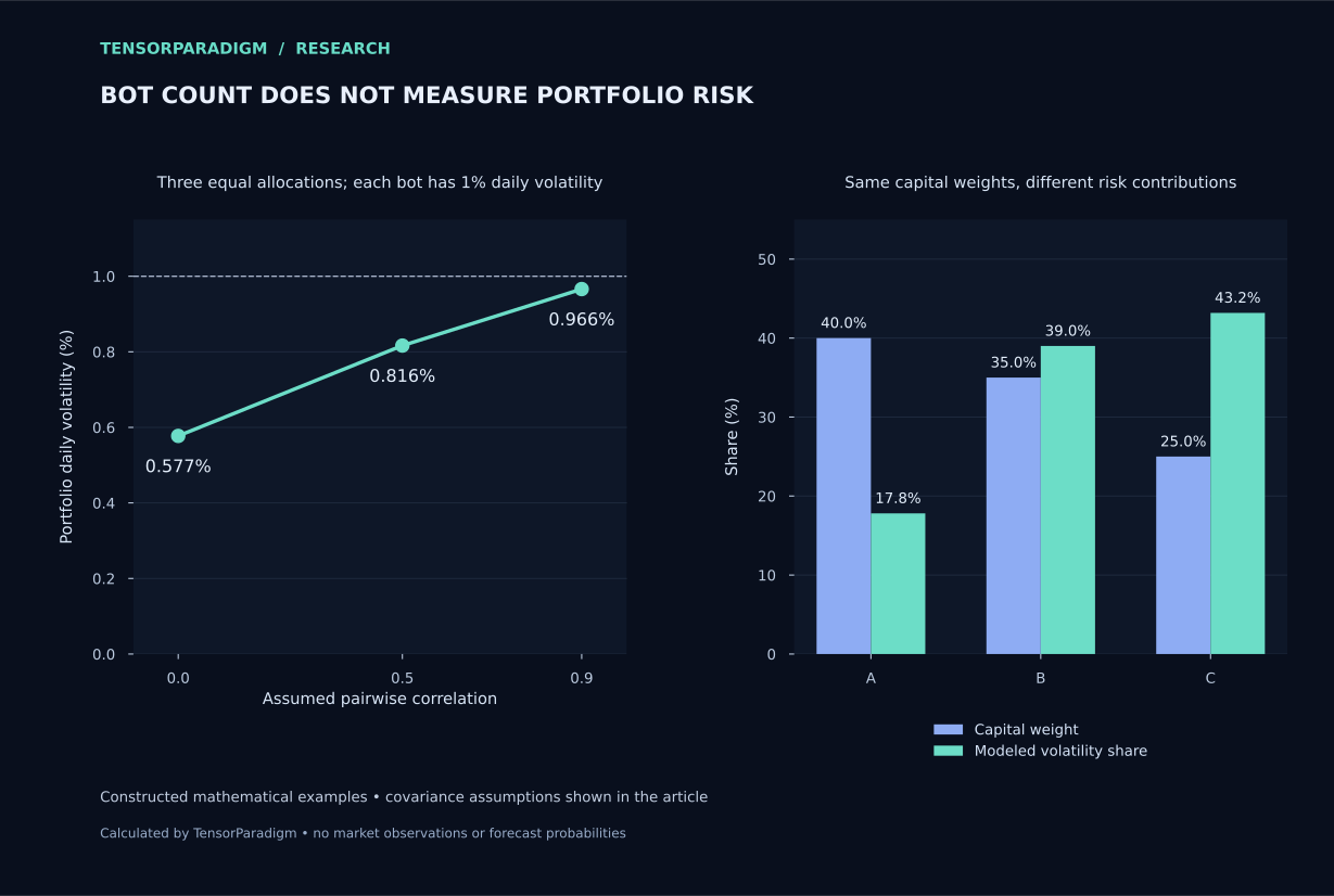
A smaller two-bot example makes the distinction intuitive. Equal capital in uncorrelated streams with 2% and 1% daily volatility produces 1.11803% portfolio volatility and 80%/20% risk shares. Equal money does not produce equal contribution to variance. Neither example establishes that equal risk would be the best allocation for a real account.

Treat the correlation estimate as a measurement with a context

For real bot records, display the sample dates and count alongside each estimate. Compare prespecified windows and investigate changes in trading rules, market exposure, volatility and activity. A stream with many genuine cash days can have a different full-period relationship from its relationship while both bots are active. Report the question each version answers rather than selecting whichever matrix looks most diversified.

Stress-period and downside diagnostics are useful, but selection changes the statistic. Ang and Chen show both asymmetric comovement in their historical equity data and the difficulty of interpreting correlations calculated after conditioning on particular returns. A higher correlation on selected losing days alone does not prove that a stable process changed or that contagion occurred. Show the selection rule, observations and dates. [4]

Optimization adds another layer of selection. Choosing among many bots and weight combinations can exploit error in estimated covariances as well as recent returns. Ledoit and Wolf’s covariance-estimation work explains the motivation for shrinkage when a sample matrix is noisy; their equity-portfolio evidence is not a guarantee about a particular bot allocation. [3]

Before adopting an allocation rule, define the history it can see, its review schedule, turnover constraints and how it will be evaluated afterward. Repeatedly increasing the weight of the latest winner is itself a trading strategy. It needs a later test with its rebalancing costs and decisions recorded. This article does not fit an optimizer or claim to identify optimal weights.

Stress the loss that the correlation matrix cannot describe

Keep a position-level view next to the return matrix. Record the instrument, direction, size, venue, collateral and pending orders for each bot. Different entry signals can still produce the same long exposure. Opposite positions can produce small net exposure while leaving large gross exposure, funding, basis and execution demands—where the venue actually retains both legs. Some account modes net the same instrument instead, which changes bot-level ownership and reconciliation.

For a transparent joint-loss calculation, assume our 100,000-USDT account starts the scenario at 40/35/25 weights and the three sleeves lose 8%, 6% and 10% at the same time. The account loses 7,800 USDT, or 7.8%. This is an assumed one-period scenario at explicitly stated weights, separate from both the fixture and the covariance examples. No event probability or historical quantile is assigned.

An equal-capital split loses 8,000 USDT under these particular shocks. Holding 20% in zero-return cash and proportionally scaling the risky allocations to 32/28/20 reduces the assumed loss to 6,240 USDT. The smaller loss comes from less risky capital in this scenario. It is not evidence that the remaining strategies became less dependent, or that 20% cash is an optimal reserve.

Extend the scenario to the actual account: wider spreads when exits coincide, a missing hedge, repriced collateral, higher required margin and delayed access to a venue. Define whether each cost is already inside the assumed sleeve return before adding it again. A linear fully funded sleeve-loss example does not price options, funding paths, liquidation mechanics or a stablecoin failure.

Clearing practice illustrates why this broader view matters. CME’s SPAN 2 framework distinguishes historical risk, stress risk, liquidity and concentration. We use that as a reason to examine multiple dimensions of an account; our scenario is not a reproduction of CME margin or a broker’s required collateral. [6]

Bots also share collateral, infrastructure and failure modes

A statistical result does not entitle the account to a margin offset. CME’s equity-product SPAN 2 filing describes offsets constrained by eligible groups and an economic basis. That is a specific clearing methodology, not a promise about a retail broker or crypto exchange. Check the rules for the actual account, contracts and collateral. Separate software processes do not create independent collateral pools. [7]

As a named broker example, Interactive Brokers describes real-time margin calculations and liquidation when relevant requirements are not met for specified margin account types. The trigger belongs to the account’s rules, not to each bot’s preferred stop. Product and jurisdiction details matter; this article supplies no universal margin threshold. [8]

Operational concentration can survive excellent return diversification. Several bots may depend on one exchange, one data vendor, one cloud region or the same authentication service. An independent signal does not keep an inaccessible order route working. Record these dependencies as design exposures and rehearse the account’s response; a return-correlation coefficient has no column for them.

The same issue appears during recovery. A restarted bot that remembers its last signal but not an already filled order can create a duplicate position. Before resuming, reconcile broker positions, open orders, fills, sequence identifiers and the central risk ledger. A green process-health indicator is not proof that account state agrees.

Give account limits authority over every bot’s next order

A shared account needs a shared decision about whether a proposed order is allowed. Before releasing a risk-increasing order, reconcile the current book and reserve the cash, margin or exposure it may consume. The check and reservation must be coordinated across simultaneous bot requests. Otherwise two individually acceptable orders can both pass against the same unreserved capacity.

Separate a block on new risk from cancellation, position reduction and liquidation. They are different actions. A block leaves existing positions exposed. Cancelling all orders can also remove protection. A flattening instruction creates orders whose fills and failures still need reconciliation. Define how risk-reducing orders remain possible under the chosen state and avoid treating one generic “kill switch” as a complete policy.

Set limits from the account’s mandate, product constraints and stress tolerance, then specify who can change them and what must happen before restarting. We do not derive a universal daily-loss limit or stop level from the constructed 24-day fixture. A threshold is an operational trigger; gaps, unavailable markets and execution costs can carry the realized loss beyond it.

The table gives a control design to adapt, not recommended numeric thresholds. It becomes useful when each row has an owner, a data source, an action that can actually execute and a recorded recovery condition.

Evaluate the next bot as a change to the account

The acceptance question is whether the candidate improves the account under a stated objective and feasible operation. Compare the current account and the proposed allocation at explicit capital and exposure assumptions. Include any cash displaced, extra turnover, infrastructure cost and margin requirement. A high standalone Sharpe ratio does not settle that comparison.

Begin with a documented shadow allocation. Record its version, proposed sizes, contemporaneous inputs and the decisions the allocator would have accepted or rejected. Retain skipped signals. A paper account can still be optimistic about fills, so model execution assumptions explicitly and compare them with observed quotes or later small-scale execution if that is separately authorized.

If you use Monte Carlo or bootstrap diagnostics, keep the bots together when sampling. Resample the synchronized return vector, and preserve appropriate time blocks if serial dependence is part of the question. Independently shuffling every bot destroys the co-loss relationships you set out to measure. Such resampling remains conditional on its input and does not recreate strategy decisions, liquidity or absent crises. We have not run that additional experiment for this article.

ChatGPT or Claude can help reconcile exports and explain a risk report; Codex or Claude Code can help build the reporting software. Give the assistant explicit units, timestamps and accounting identities. The reusable prompt below asks for an auditable diagnostic rather than a profitable allocation invented from a short sample. The supplied exercise was implemented with AI assistance and checked through executable arithmetic tests; it is not a comparative experiment between AI products.

Review these timestamped bot returns, marked positions, account balances and outstanding orders. Reconcile bot capital to actual account equity. Identify missing or stale records before calculating common-sample return correlations and covariance contributions at stated weights. Show shared market, collateral and infrastructure exposures. Calculate the specified joint shocks in account currency; do not invent probabilities or optimize the allocation. Separate observed records, assumed scenarios and unresolved questions. Return the formulas, source record IDs and a reproducible report.

Make the decision with a reconciled account, not a bot count

The examples resolve several common misconceptions. Three bots can have little modeled diversification when their assumed correlations are high. A small capital sleeve can dominate modeled volatility. A modest correlation does not exclude simultaneous losses. Combined drawdown must come from combined equity, and a cash buffer changes the amount exposed rather than the strategies’ statistical independence.

For an existing portfolio, the next useful deliverable is a short account report: reconciled equity, capital and risk contributions, current signed and gross exposures, joint stress losses, operating dependencies and the state of each account-level control. When a field cannot be verified, keep it unresolved instead of replacing it with a reassuring estimate.

Adding another bot is justified by what it contributes to that report and to the account’s objective. The research can support keeping it small, changing the allocation, investigating the records or declining the addition. The ability to reject an apparently attractive standalone bot is a useful outcome of portfolio analysis.