How to Backtest Machine Learning Trading Strategies in Python Without Lookahead Bias
An executed Python ML backtest: mature labels, monthly training, causal tests, actual trade accounting and a losing result after costs. Six features, no future inputs.
Backtest an ML trading strategy by reconstructing what was available at each decision: completed features, already resolved training labels, training-only preprocessing and orders filled after the signal. We executed that procedure for a daily Bitcoin logistic-regression strategy. It returned −1.67% after modeled costs in 2024–25, against +96.28% for an initial-allocation buy-and-hold baseline. A deliberately invalid version that consumed future returns appeared to earn +867.06%. The difference shows why the information calendar must be tested before interpreting profitability.
WHAT THIS INVESTIGATION ESTABLISHES
- A chronological split can still leak: five training rows at each monthly boundary had labels that had not finished yet.
- A fresh scaler and model were fitted monthly on eligible past rows; earlier evaluation labels entered later fits only after becoming observable.
- Changing future observations left the valid implementation’s earlier forecasts and orders identical, while the invalid control failed.
- The fixed strategy made +17.51% without fees or slippage, then lost −1.67% after costs over 66 completed trades.
- Forecast scores, a losing trade, nine development variants and conditional bootstrap paths explain why this result does not justify live capital.
Start with a timestamp, then ask whether the prediction was possible
Our earlier lookahead-bias guide explains common failure modes. This investigation builds and executes an actual fitted ML pipeline, then follows its predictions into a cash account. The question is specific: do six completed daily price and volume features help a simple model choose profitable five-day Bitcoin trades after costs?
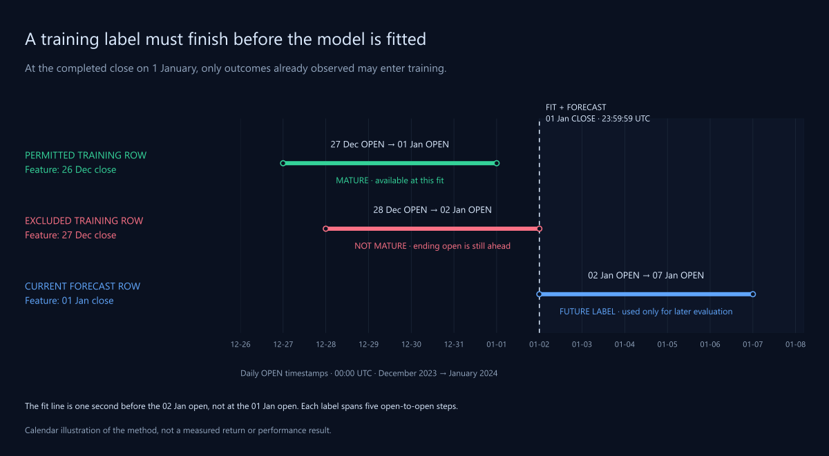
The first useful check is a concrete acceptance example. At the completed close of 1 January 2024, the latest eligible training feature date is 26 December 2023. Its outcome runs from the 27 December open to the 1 January open, so it is already known. The feature row dated 27 December needs the 2 January open and must be excluded. Our executed fit contains 725 rows, ends on 26 December and predicts 0.452770 for the 1 January feature row: below the fixed 0.55 trading threshold.
If a purported reproduction fits through 31 December, investigate the label-end filter before comparing profit. If it predicts a different probability, compare the UTC daily input, feature order, scaler statistics and package versions. This gives a debugging target near the beginning, rather than asking readers to trust an attractive final curve. The full implementation, protocol, attributed input, fit records and trade ledger are retained in the repository research records.
Freeze the hypothesis and the account rules before measuring returns
The economic hypothesis is deliberately modest: recent returns, volatility, range and relative activity may contain enough information about the next five open-to-open days to compensate for repeated round-trip costs. A logistic regression is transparent enough to inspect coefficient by coefficient. The hypothesis is plausible to test; it is not evidence of an edge.
We recorded the protocol and configuration before calculating this study’s performance. C = 1 and the 0.55 threshold were fixed, not chosen from the best result. The limited development grid is disclosed later. Development and evaluation prices had already appeared in earlier TensorParadigm projects, so this is a retrospective method demonstration, not an untouched discovery sample.
| Decision | Fixed specification |
|---|---|
| Market and clock | BTCUSDT; daily UTC; spot-like long/flat cash account |
| Forecast | At completed close t; probability that open[t+6] / open[t+1] − 1 > 0 |
| Training | Monthly; previous 730 calendar days; only resolved labels; at least 252 complete rows and both classes |
| Model | StandardScaler → LogisticRegression; C = 1, lbfgs, max_iter = 2000 |
| Entry and exit | Flat, p ≥ 0.55: buy at open t+1; sell at open t+6; no signal on the exit-fill day |
| Sizing | 90% of available cash including entry fee; fractional BTC; one position; no leverage |
| Costs per side | 10 basis points fee; 5 basis points adverse fill; no additional spread deduction |
| Development | 2021; 365 daily bars; earlier 2020 observations provide initial training |
| Validation | 2022–23; 730 bars; annual cold-start folds also reported |
| Evaluation | 2024–25; 731 bars; monthly refit procedure and settings frozen |
Every period starts with 10,000 USDT and no position. A scheduled five-day exit remains an exit even when the next model forecast disagrees. The last permitted entry signal is determined by the known calendar, so every strategy trade can finish within its reporting period. The final six dates can have forecasts but cannot initiate a trade or contribute an unresolved outcome to the period’s classification scores.
Establish what the data represent, including what remains unverified
The input contains 2,142 complete daily candles from 20 February 2020 through 31 December 2025. We reuse the humblefool06 BTC-USDT four-hour archive at revision 9f491eb5340dd6a24f27fde24edf098e1e785443, whose publisher declares CC BY 4.0. Daily bars combine six UTC observations: first open, maximum high, minimum low, last close and summed base volume. The preceding incomplete day is excluded. The normalized CSV’s SHA-256 is 43655a51e6cb41c2ee087bd947f4cefb7dd4151617a29d7f75a3cda471ae5cbb. [5]
An earlier study’s retained 18 October 2026 cross-check matched all 731 evaluation-period candles, or 3,655 OHLCV cells, to Binance’s daily endpoint using decimal comparison. We inherit that record with the same input; we did not perform a new independent audit for this article. The archive does not explicitly identify its upstream venue. Matching Binance establishes price agreement, not independent venue coverage or upstream attribution. The 2020–23 training and validation observations remain externally unverified. Binance identifies candles by their opening timestamp; a daily date in our tables names the UTC session. [6]
The program checks unique ascending dates, uninterrupted daily spacing, finite OHLCV, positive prices and consistent high/low bounds. Those checks catch malformed input, not every bad observation. This single surviving crypto instrument also says nothing about the performance of an historically investable universe. Python 3.13.3, pandas 2.2.3, NumPy 2.2.6 and scikit-learn 1.6.1 produced the reported calculations.
Use future prices to define outcomes, never to supply a forecast input
The six inputs are one-, five- and twenty-day close returns; the population standard deviation of the latest twenty one-day returns; the completed day’s high–low range divided by its close; and volume divided by its trailing twenty-day mean minus one. All windows include the just-completed session. We discard incomplete warm-up rows rather than backfill them. A current close is a valid input for a decision after that close; it is unavailable for a decision at the same day’s earlier open.
The following feature expressions are excerpts from the executed Python implementation. A trailing window is essential. Replacing it with a centered window or estimating a transformation on the full history would change the information available at the decision. Scikit-learn’s leakage guidance likewise requires learning transformations from the training subset. [1]
returns = close.pct_change(fill_method=None)
X = pd.DataFrame({
    "return_1": returns,
    "return_5": close.pct_change(5, fill_method=None),
    "return_20": close.pct_change(20, fill_method=None),
    "volatility_20": returns.rolling(20).std(ddof=0),
    "range_to_close": (high - low) / close,
    "relative_volume_20": volume / volume.rolling(20).mean() - 1,
})
The target uses future opens because it describes the outcome being predicted. Label 1 means the raw exit open exceeds the raw entry open; equality is class 0. It does not mean the trade made money after fees. The negative shifts below belong only in target construction. The missing final outcomes remain missing: applying a comparison alone would silently turn unknown outcomes into false class-0 observations.
target_return = open_price.shift(-6) / open_price.shift(-1) - 1
y = (target_return > 0).where(target_return.notna())
label_end = X.index + pd.Timedelta(days=6)

train_mask = (
    (X.index >= fit_date - pd.Timedelta(days=730))
    & (X.index < fit_date)
    & (label_end <= fit_date)
    & y.notna()
    & X.notna().all(axis=1)
)
A date split is insufficient when training labels extend into the future
At the 1 January 2024 close, a naïve previous-730-days filter selects feature dates from 1 January 2022 through 31 December 2023. Five of those rows are ineligible: their outcomes end on 2–6 January 2024. The maturity condition removes them, leaving 725 observations through 26 December. The same five-row exclusion appears at each monthly fit in the evaluation record.
The diagram distinguishes an outcome already observed from one that crosses the decision boundary. Its dates describe the actual protocol, not an invented price path. Although both sides of the boundary are called January in prose, the 1 January open is available at that day’s close; the 2 January open is not.
For this complete daily calendar, a TimeSeriesSplit whose first test feature has date t would need a five-sample gap to make the final training feature t−6. A six-sample gap would be conservative. Scikit-learn defines gap in samples, not elapsed calendar time. Variable holding periods, missing sessions and delayed data require actual availability timestamps instead of copying this integer. We used explicit label-end masks, not TimeSeriesSplit, for the recorded fits. [2]
This forward trading experiment must preserve chronology. That does not make a universal claim about every use of random cross-validation in time-series statistics. Here, adjacent five-day outcomes overlap, and a row dated before the test set can still contain an unavailable target. Removing the training boundary leak also does not make the remaining test outcomes statistically independent.
Fit the scaler and the classifier inside the same eligible training window
On the first forecast day of each month we create a fresh pipeline, fit it only on the mature trailing rows and retain its state until the next monthly fit. Today’s feature row is transformed with those fitted statistics; it is not added to the scaler fit. A pipeline helps enforce that boundary but cannot repair a future-derived feature or an incorrectly selected training set. [1]
pipeline = Pipeline([
    ("scale", StandardScaler()),
    ("model", LogisticRegression(
        C=1, solver="lbfgs", max_iter=2000, random_state=6142026
    )),
])
pipeline.fit(X.loc[train_mask], y.loc[train_mask].astype(int))
assert pipeline.named_steps["model"].classes_.tolist() == [0, 1]
p_up = pipeline.predict_proba(X.loc[[signal_date]])[0, 1]
C is the inverse regularization strength: a smaller value imposes stronger regularization. The positive probability column is checked against classes_ = [0, 1]. We record feature order, training-row hash, scaler means and scales, coefficients, intercept and optimizer iterations. The lbfgs solver is used; passing random_state does not explain its determinism. [3]
Monthly refitting legitimately uses earlier evaluation outcomes after they mature. For example, a February fit can learn from eligible January observations. This is a fixed updating procedure evaluated forward in time, not a single model frozen for two years. We never used later evaluation results to change C, the threshold, features or refit schedule. Retuning those choices would require a new evaluation protocol.
Reconstruct the first accepted prediction instead of trusting predict_proba
The first accepted evaluation signal occurs at the 12 January 2024 close. It still uses the 1 January fit: 725 rows from 1 January 2022 through 26 December 2023, with the latest training outcome ending at the 1 January open. The table exposes the actual feature vector, its training-standardized values and the fitted coefficients. Values here are rounded; the audit uses full precision.
| Feature | Raw value | Standardized z | Coefficient |
|---|---|---|---|
| return_1 | −0.076748 | −2.672794 | −0.103549 |
| return_5 | −0.026094 | −0.417899 | −0.111867 |
| return_20 | −0.021039 | −0.200837 | +0.039253 |
| volatility_20 | 0.030521 | 0.420563 | +0.026111 |
| range_to_close | 0.117233 | 2.754973 | −0.019805 |
| relative_volume_20 | 0.778955 | 1.552860 | +0.037502 |
For each feature, z = (x − training mean) / training scale. The intercept 0.014133035 plus the sum of z times coefficient gives a logit of 0.344416426. Applying 1 / (1 + exp(−logit)) gives 0.585262925. That exceeds 0.55, so a flat account submits a buy for the 13 January open. This is a probability of a positive gross price move under the model, not a calibrated probability of net trading profit.
The first evaluation-day probability, 0.452769888, correctly produces no trade. These two audit points help distinguish a feature or fitting discrepancy from an order-handling discrepancy. A correct prediction can still be converted into an incorrect backtest if its fill, cash sizing or exit clock is wrong.
Keep the forecast, order and cash account separate
An eligible close signal schedules a next-open entry and an exit five open-to-open days later. The simulation allocates cash at the actual fill: quantity = 0.90 × cash / (buy fill × 1.001). This describes broker-side cash allocation, not a quantity calculated yesterday using tomorrow’s unknown open. Buy fill equals raw open × 1.0005; sell fill equals raw open × 0.9995. Each fee is 0.001 times slipped notional.
if flat and not exited_today and p_up >= 0.55:
    entry_date = signal_date + pd.Timedelta(days=1)
    exit_date = signal_date + pd.Timedelta(days=6)
    if exit_date <= evaluation_end:  # known calendar, not future prices
        pending_buy = (entry_date, exit_date)

# At the entry open:
fill = open_price * 1.0005
quantity = 0.90 * cash / (fill * 1.001)
At every daily close, equity equals cash plus BTC quantity times the raw close. Drawdown is measured from the running peak of this daily-close account, including the initial balance. Slippage is already embedded in prices and is not deducted again. Strategy positions all finish within the reporting window; buy-and-hold instead retains BTC at the final close, with its entry fee included and no fictional exit fee.
Crypto’s daily close and next open are adjacent. A fill exactly at that next open is an idealized assumption: this study does not establish achievable model-computation, exchange or network latency. Five basis points is a sensitivity assumption, not an observed order-book measurement. We exclude leverage, shorting, stops, funding, cash interest, taxes, fixed operating expenses and USDT conversion; fractional quantities ignore venue filters. These choices define the simulation’s scope.
The fixed model loses after costs and trails the simple holding baseline
Gross results come from a separate account run with both fees and slippage set to zero. Net results use the fixed ten-plus-five-basis-point assumptions per side. Development, validation and evaluation accounts each start at 10,000 USDT. The table reports measured results, not fitted expectations.
| Period | Gross ML return | Net ML return | ML max drawdown | Closed trades | Net buy-and-hold |
|---|---|---|---|---|---|
| Development 2021 | +26.88% | +10.56% | 41.81% | 51 | +53.60% |
| Validation 2022–23 | −40.06% | −46.76% | 54.13% | 44 | −7.78% |
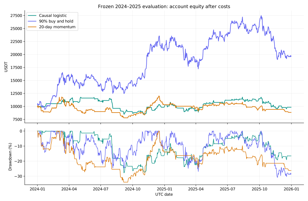
| Evaluation 2024–25 | +17.51% | −1.67% | 27.82% | 66 | +96.28% |
During evaluation the ML account finishes at 9,832.51 USDT, with no open BTC and −167.49 USDT of completed-trade P&L. Its 27.82% maximum daily-close drawdown is only modestly below buy-and-hold’s 30.86%, despite average invested exposure of 40.63%. It holds BTC on 330 of 731 daily closes. Lower exposure does not automatically imply an attractive risk-adjusted alternative.
Two decision-policy baselines use the same five-day holding, cooldown, sizing and cost rules. Buying when the completed twenty-day return is positive returns −11.63% over 71 trades, with 33.99% drawdown. Trading when the monthly mature training sample’s positive-label frequency reaches 0.55 returns −26.56% over 36 trades, with 37.85% drawdown. The ML rule beats these two policies here, but loses money and badly trails the holding baseline. That is insufficient evidence that its features add a durable economic advantage.
The plotted accounts use actual calculated daily equity. Buy-and-hold invests 90% at the first period open with the same entry costs and leaves 10% cash. Its much greater market exposure is part of the comparison, not a controlled estimate of ML’s causal contribution. For broader interpretation, see our ML versus rule-based trading investigation.
Prediction accuracy is a different measurement from trade profitability
We score 725 fully observed evaluation forecasts, including forecasts made while the account already holds BTC. The remaining six outcomes extend beyond the period and are excluded. There are 390 positive labels, or 53.79%. The frequency baseline predicts each month’s mature training positive fraction without using the six features.
Accuracy uses a 0.50 classification cutoff; orders use 0.55. Brier score measures squared probability error, log loss penalizes probability errors logarithmically, and ROC AUC measures ranking. Their values do not incorporate position sizing or fees. Lower Brier score alone also does not establish better calibration: it reflects more than calibration. Our probabilities were not separately calibrated. [4]
| Evaluation forecast | Accuracy at 0.50 | Brier ↓ | Log loss ↓ | ROC AUC |
|---|---|---|---|---|
| Six-feature logistic regression | 50.76% | 0.251416 | 0.695919 | 0.502044 |
| Mature training-frequency baseline | 53.79% | 0.249933 | 0.693033 | 0.476881 |
The ML model does not improve on the frequency baseline’s Brier score or log loss. Its AUC of 0.5020 is close to 0.5, but we do not attach an independent-observation significance claim to these overlapping outcomes. Nor is 725 forecasts equivalent to 725 independent trades: the account actually closes 66 trades. The small scoring differences provide no compelling predictive case to counter the economic result.
Follow the first losing trade through both fills and the cash balance
The 12 January forecast of 0.585262925 triggers the first trade. On 13 January, the raw entry open is 42,782.74 USDT. After five basis points of adverse execution, the buy fill is 42,804.131370. Quantity is 0.210050027959 BTC. Entry notional is 8,991.008991 USDT and the fee is 8.991009, leaving exactly 1,000 USDT cash.
The mandatory 18 January exit uses the raw open of 42,776.09 and a sell fill of 42,754.701955. Its fee is 8.980626 USDT. Price P&L between slipped fills is −10.382650; subtracting the two fees gives −28.354285 USDT. Final cash is 9,971.645715. This reconciles with the initial 10,000 and a flat position; the model’s probability did not override the scheduled exit.
Across all 66 evaluation trades, 32 win and 34 lose after costs: a 48.48% win rate. The average winner is +332.83 USDT and the average loser −318.18, a payoff ratio of about 1.05. The average trade is −2.54 USDT and profit factor is 0.9845. Neither the win rate nor the gross direction forecast alone explains the cash result; fees, fill prices, varying capital and payoff size do.
Make a leaking model fail a test, even when its returns look excellent
We changed every observation after 15 June 2024: OHLC prices doubled and volume tripled, while all earlier values stayed fixed. Rebuilding the valid model left past features, eligible training matrices, scaler/model state, forecasts, decisions and fills unchanged. The maximum earlier probability difference was exactly zero. This is an executed invariance check for this implementation; it is not proof that every possible bias has been eliminated.
changed = bars.copy()
future = changed.index > cutoff
changed.loc[future, ["open", "high", "low", "close"]] *= 2
changed.loc[future, "volume"] *= 3
# Valid: past features, fit states, predictions and orders are identical.
# INVALID control: X also contains target_return, so this check fails.
The negative control deliberately adds the realized future open-to-open return as a seventh input. It retains the same monthly pipeline and account rules but violates information availability at prediction time. It reports an apparent +867.06% net return, 97.66% classification accuracy and 0.998676 AUC. These are measurements of an INVALID backtest, not a strategy candidate or a result used in selection.
The same future mutation changes the invalid model’s earlier probabilities by as much as 0.998626629. The control demonstrates that a clean scaler, chronological fitting and plausible order accounting cannot rescue an unavailable input. By contrast, the five immature boundary labels are a quieter error: the calendar proves them invalid without requiring an eye-catching performance change.
The research tests also cover trailing feature timing, terminal missing labels, exact label-maturity boundaries, training-only scaling, monthly fit reuse, classification-period boundaries, non-overlapping orders, exit-day cooldown, fee-inclusive sizing, cash/P&L reconciliation and deterministic block resampling. A causal test should fail on a known broken version; simply observing that the code runs is weak evidence.
Disclose the development grid and preserve the disappointing validation folds
We evaluated only nine development combinations: C in {0.1, 1, 10} and entry threshold in {0.50, 0.55, 0.60}. The table shows net 2021 returns. Every variant is retained, including those that lose appeal when the threshold changes. The predeclared C = 1, threshold = 0.55 configuration remains the article’s strategy even though other development settings look better.
| C | Threshold 0.50 | Threshold 0.55 | Threshold 0.60 |
|---|---|---|---|
| 0.1 | +7.81% | +10.56% | +25.24% |
| 1 | +7.81% | +10.56% | +55.01% |
| 10 | +7.81% | +10.56% | +55.01% |
At thresholds 0.50 and 0.55, all three C values produce the same executed trade path; this does not mean their probabilities are identical. At 0.60, the C = 0.1 path differs. Threshold changes alter trade eligibility and subsequent cooldown opportunities, explaining why small forecast differences can change compounded returns. This grid does not identify a stable profitable region across market periods.
Validation uses the fixed procedure, with monthly rolling fits. Separate annual accounts lose −44.04% in 2022 over 37 trades and −4.87% in 2023 over seven trades. Their maximum drawdowns are 54.13% and 8.60%. These are cold-start folds with their own final calendar exclusions, so compounding their returns is not exactly the continuous 2022–23 account. In the continuous evaluation account, 2024 returns −1.14% and 2025 −0.54%.
Selecting the best historical variant creates a different research procedure from evaluating one fixed rule. Bailey and coauthors formalize how selection among backtests can lead to overfitting. We disclose this small grid and the unfavorable folds; we do not claim to estimate a formal probability of backtest overfitting from nine settings. Changing the configuration after this report would turn these periods into development evidence. [7]
Turnover consumes the gross gain, and a few trades matter substantially
The evaluation account executes 132 fills. Summed buy and sell notional is 122.29 times initial equity; this one-way turnover definition includes both sides and is not 122 complete rotations of the whole account. Fees total 1,222.92 USDT. Embedded execution shortfall relative to the raw opens totals 611.46 USDT. Changing costs also changes later position quantities, so subtracting those ledger totals from the separate gross account is not an exact way to reconstruct the net result.
The sensitivity table changes only adverse slippage while keeping the ten-basis-point fee per side and the same model decisions. Even zero slippage produces only +4.34%; ten basis points gives −7.34%. This study therefore does not establish a comfortable execution margin. The fee-and-slippage-free result of +17.51% is informative about the accounting, not an attainable forecast of net returns.
| Fee per side | Slippage per side | Net evaluation return | Max drawdown |
|---|---|---|---|
| 10 bp | 0 bp | +4.34% | 27.37% |
| 10 bp | 5 bp | −1.67% | 27.82% |
| 10 bp | 10 bp | −7.34% | 28.27% |
| 10 bp | 20 bp | −17.72% | 30.67% |
The three largest net winning trades contribute +2,764.12 USDT. All other completed trades sum to −2,931.61. This is a descriptive concentration calculation using the observed ledger, not a rerun in which those trades disappear and later cash changes. A proposed improvement should explain how it would retain gains or reduce turnover using information available beforehand; deleting historical losers would merely create another biased result.
Resample account paths without pretending to manufacture new evidence
We generated 5,000 conditional paths by drawing circular blocks of twenty consecutive net daily account returns, including flat days, until each path contained 731 days. Seed 6142026 fixes the calculation. Wrapping at the sample end and keeping consecutive blocks preserves some local dependence, using the circular resampling construction described by Politis and White. Our block length is fixed at twenty days; we did not use their automatic selection method. This choice does not guarantee that all relevant dependence is captured or that the return process is stationary. [8]
The fifth percentile, median and ninety-fifth percentile of terminal return are −42.11%, −1.03% and +61.61%. For maximum drawdown they are 16.79%, 30.26% and 51.19%. Of the resampled paths, 51.44% finish below starting equity. That fraction is conditional on the historical sample and resampling rule; it is not an estimated real-world probability that this strategy will lose money.
This bootstrap rearranges the realized account return series. It does not regenerate prices, refit the model or recompute orders, and its sampled sequences need not be feasible trading histories. It explores path sensitivity conditional on what happened. More resampled paths reduce simulation noise but add no new market observations, independent trades or evidence of predictive advantage.
Give the AI collaborator acceptance conditions it can actually check
ChatGPT or Claude can help turn a trading idea into a precise specification and challenge ambiguities. Codex or Claude Code can work with repository files, execute calculations and inspect failures. Official product documentation supports these development roles; none of those capabilities establishes a trading edge. This project used Codex assistance and local Python calculations. We did not run a controlled ChatGPT-versus-Claude comparison, use an LLM to produce market forecasts or obtain independent expert review. [9] [10]
The prompts below make four different jobs reviewable. Supply the frozen specification and relevant code with each request. Market data supplies observations, executable programs calculate results, and the researcher decides whether assumptions and evidence justify a new test. A confident narrative cannot substitute for a reconciled ledger. For the broader development process, see building and testing a trading algorithm.
Specify a daily UTC BTCUSDT long/flat ML experiment. Forecast at completed close t the sign of open[t+6]/open[t+1]-1. Define each feature’s availability, target maturity, monthly training window, entry/exit calendar, cash sizing and costs. Separate refitting from hyperparameter selection. List ambiguities and give the latest eligible training feature date at the 2024-01-01 close. Do not calculate performance or choose settings from returns.Implement the attached frozen specification with separate feature/label, monthly-fit and cash-account functions. Fit StandardScaler only inside the mature training slice. Preserve missing terminal labels. Record eligible dates, feature order, scaler state, coefficients, probabilities, decisions and fills. Do not retune C=1 or threshold=0.55. Add a test where future OHLCV changes leave every earlier valid prediction and order unchanged; show that an intentional target_return feature fails it.Audit the 2024-01-12 signal without changing the strategy. Reconstruct its standardized features, logit and probability from the 2024-01-01 fit. Trace the 13 January entry and 18 January exit using ten-basis-point fees and five-basis-point adverse fills. Show quantity, cash, both fees and net P&L. Reconcile final equity with initial cash plus closed and open marked P&L. Identify the first divergent record, rather than explaining only the final return.Write a research report from the recorded outputs. Include every development variant, chronological periods, gross/net returns, baselines, forecast scores, drawdown, exposure, turnover, trade asymmetry, costs and concentration. Explain overlapping labels and conditional block-bootstrap limits. Mark the future-feature control INVALID wherever reported. Distinguish executed calculations from illustrative excerpts and unexecuted components. Disclose prior price familiarity and data-verification limits. Do not optimize to obtain a winning headline.For this rolling scikit-learn pipeline, we did not provide or execute a matching Pine implementation. Copying one fitted month’s coefficients would freeze a different strategy; a faithful comparison must reproduce the training window, scaling, label maturity, refits and execution semantics. This is a scope limit of the investigation, not a claim that Pine cannot express machine-learning calculations. Our Python–Pine backtesting study explains why matching a signal formula alone is insufficient.
The justified next step is a recorded prospective test, not deployment
The implementation passes the causal properties we tested, but the fixed strategy loses after costs, fails to improve the main probability scores and suffers a severe validation drawdown. Those findings do not justify live capital. The article’s useful result is a method for distinguishing valid historical measurement from a profitable-looking information leak.
If continuing the research, record a new prospective paper-trading interval before it begins. Freeze the feature set, maturity rule, refit calendar, costs and reporting criteria. Timestamp each completed input, fitted state, signal and feasible next execution; measure actual delay and quoted spread. Compare against both the training-frequency forecast and the simple holding account. Preserve every proposed variant and assign later data to evaluation only after its outcome matures.
A lower-turnover design is a reasonable new hypothesis because costs materially change this result, but it must earn its own later test. Reusing 2024–25 to pick a different threshold or holding period makes those dates development data. One market, externally unverified earlier data, dependent outcomes, idealized fills and no live execution limit what this investigation can establish. Passing a lookahead check is necessary for interpreting a backtest; profitability still requires separate evidence.
A review checklist for an ML trading backtest
- For one real prediction, identify the exact observation, fit, decision and fill timestamps.
- Show that every training target had resolved before its fit; do not rely on feature-date order alone.
- Fit transformations on eligible training rows, preserve feature order and retain each monthly model state.
- Keep unresolved terminal labels missing, and distinguish forecast scoring from executed trades.
- Make future perturbations leave earlier outputs unchanged, and verify that a known leaking control fails.
- Reconcile both fill costs and cash, including open marked positions and slippage embedded in prices.
- Report all tried settings, unfavorable periods, suitable baselines and sensitivity to realistic costs.
- Freeze the next prospective procedure before observing the evidence that will judge it.
Practical questions about ML backtesting
Does a chronological train/test split prevent lookahead bias?
It prevents some future-to-past mixing, but it is insufficient. A training row before the boundary can have an outcome that ends afterward. Our five-day target requires excluding five immature rows at each fit. Preprocessing, feature availability and order timing also need separate checks.
Should every feature be shifted by one day?
No. Timing determines the required shift. Today’s completed close and total volume can support a signal after today’s close for a later fill. They cannot support an order at today’s earlier open. Blindly shifting all inputs can change the intended strategy without resolving other leaks.
Can an evaluation-period observation enter a later monthly training set?
Yes, if the updating procedure was fixed beforehand and the observation’s target has matured by that fit. That simulates an operational model learning from newly available history. Changing hyperparameters after inspecting evaluation results is a different selection decision and needs new evaluation evidence.
Does a predicted probability above 0.55 mean the trade has positive expected profit?
No. Our label describes a positive raw five-day open-to-open return. Net expectancy also depends on gains and losses, costs, capital and execution. The model’s probabilities were not separately calibrated, and its valid strategy lost after modeled costs.
How much gap should TimeSeriesSplit use for trading labels?
Derive it from actual label availability. For our complete daily data and a close-t decision, the latest training feature is t−6, equivalent to a five-row gap before the first test feature t. Other targets, session calendars and reporting delays can require a different gap or explicit timestamp filtering.
Can ChatGPT or Claude validate that an ML trading bot is profitable?
They can help specify the experiment, inspect code and explain recorded outputs. Profitability must come from executable calculations on correctly timed observations and then further evidence under realistic conditions. This study used Codex assistance, found an unfavorable fixed result and did not test comparative AI investment skill or live trading.
Sources and research records
Returns, model outputs and account examples are TensorParadigm’s executed calculations. Repository records retain the pre-performance protocol, configuration, attributed normalized data, runnable Python implementation, tests, all model fits and complete ledgers. The primary sources below support the methods, data and tool descriptions; they do not endorse the strategy. Scikit-learn references use the 1.6 documentation corresponding to the executed 1.6.1 environment.
- Scikit-learn 1.6: common pitfalls, training-only transformations and data leakage
- Scikit-learn 1.6: TimeSeriesSplit and its sample-based gap
- Scikit-learn 1.6: LogisticRegression configuration and probability class order
- Scikit-learn 1.6: classification and probability-scoring metrics
- humblefool06: BTC-USDT four-hour archive, pinned publisher revision and license declaration
- Binance Spot API: candlestick timestamps and market-data endpoint
- Bailey et al.: The Probability of Backtest Overfitting
- Politis and White: Automatic Block-Length Selection for the Dependent Bootstrap, including circular resampling
- OpenAI: code-generation and Codex development guidance
- Anthropic: Claude Code overview
Educational retrospective research, with modeled variable costs and idealized fills. No live trading, independent expert review or comparative AI investment experiment was conducted. Historical and resampled results do not establish future profitability.